OOF2: The Manual

3.15. The Solver Page
	Chapter 3. Task Pages

3.15. The Solver Page

The Solver Page is where it all comes together. After

Materials have been assigned to a Microstructure
a Skeleton has been adapted to it
a Mesh has been created from the Skeleton
Fields and Equations have been activated on the SubProblems
and boundary conditions have been assigned,

the Solver Page is used to find the solution to the equations.

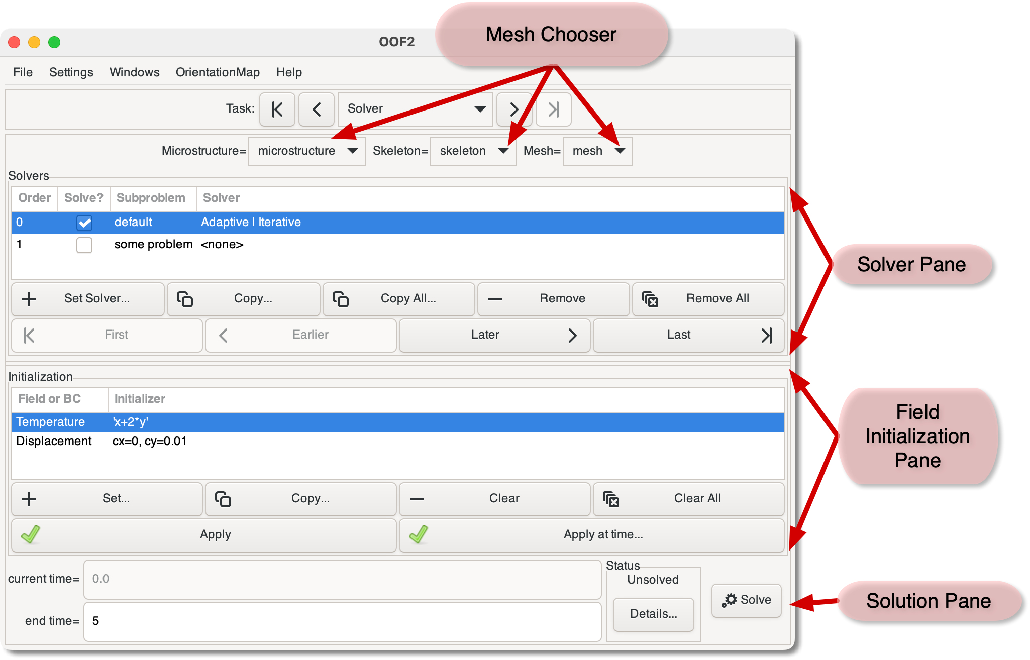
Figure 3.24 shows the layout of the Solver Page. At the top is a Mesh Chooser for selecting the Mesh to be solved. The Chooser has three parts, for selecting the Mesh and the Skeleton and Microstructure in which it resides. Below the Mesh Chooser is the Solver Pane, where solution methods are assigned to SubProblems, and below that is the Field Initialization Pane, where initial conditions are defined and applied. At the bottom of the page is the Solution Pane.

Figure 3.24. The Solver Page

3.15.1. The Solver Pane

The Solver Pane sets the solution technique that will be used for each SubProblem when the Solve button is pressed. It contains a four column list with one row for each SubProblem defined in the Mesh, and two rows of buttons that operate on the contents of the list. Clicking on a row selects it. Double clicking on a row is equivalent to selecting it and then pressing the Set Solver button. The list comprises four columns:

Order. When multiple SubProblems are being solved, they are addressed sequentially in the order given by the number in this column. The order can be changed by selecting a SubProblem and clicking one of the First, Earlier, Later, or Last buttons.
Solve? The checkbox in this column indicates whether the SubProblem should be solved or not. Clicking it invokes either the OOF.Subproblem.Enable_Solution or OOF.Subproblem.Disable_Solution commands. It's a quick way of temporarily disabling a subproblem without having to delete its solver.
Subproblem. This is just the name of the SubProblem.
Solver. This is a short hand description of the solver that has been assigned to the SubProblem. If no Solver is assigned, it will read <none>. To see the full details, select a line and click the Set button.

The buttons immediately below the SubProblem list operate on the contents of the list. Most of them require one SubProblem to be selected in the list.

Set. Assign a solver to a SubProblem via the OOF.Subproblem.Set_Solver command. The button brings up a dialog box displaying the currently assigned solver, or the default solver if no other solver has yet been assigned. The default is a static solver operating in basic mode, where OOF2 makes most of the detailed parameter choices automatically.
Copy. Copy a solver from one SubProblem to another, using the OOF.Subproblem.Copy_Solver command. The target SubProblem may be in a different Mesh.
Copy All. Copy all solvers from this Mesh to another Mesh, using OOF.Mesh.Copy_All_Solvers. Solvers will be copied only for those SubProblems that have identical names in the two Meshes.
Remove. Remove the solver from the selected SubProblem, using OOF.Subproblem.Remove_Solver. The SubProblem will not be solved until a new solver is set.
Remove All. Remove the solvers from all SubProblems, making the Mesh unsolvable until new solvers are assigned. See OOF.Mesh.Remove_All_Solvers.
First, Earlier, Later, Last. These buttons change the order of the list, by moving the selected SubProblem up (First or Earlier) or down (Later and Last). All of the buttons invoke the OOF.Mesh.ReorderSubproblems command.

3.15.2. The Initialization Pane

The Initialization Pane is in charge of assigning initial values to the Fields and floating boundary conditions that are defined on the Mesh. As explained in Section 2.5.8, initialization is a two step process: first an initializer is assigned to a Field or boundary condition, and then all the initializers are applied.

The Initialization pane contains a list with two columns: the names of the Fields (or boundary conditions) and their initializers. Items without initializers are marked with “---”. Selecting an item in the list and clicking the Set button brings up a dialog box for setting the initializers. Double-clicking on an item has the same effect.

When solving static problems, it's not necessary to initialize Fields that are active, since values will be assigned to them by the solver. However, the iterative solvers will converge faster if the initial values of the Fields are close to the actual solution. Fields and floating boundary conditions that are being used in time dependent problems should always be initialized.

Note that changing a SubProblem's solver can affect which items can be initialized. If the Equations include terms, such as mass density in the force balance equation, that contain second time derivatives, and if the solvers are not static, then the first time derivative of the relevant Fields and boundary conditions must be initialized as well. The time derivative Fields have a _t suffix in the list. For some reason, the first time derivative of a boundary condition is set differently, via an additional parameter in the Set dialog.

In Figure 3.24, Temperature's initializer has been set to a function, x+2*y, and the initializers for the two components of the displacement have been set to constants, 0.0 and 0.01.

The buttons below the list operate on the initializers in the Mesh.

Set. This button brings up a dialog box in which an initializer can be defined for the currently selected item. Clicking OK invokes the OOF.Mesh.Set_Field_Initializer or OOF.Mesh.Boundary_Conditions.Set_BC_Initializer command, depending on whether a Field or a floating boundary condition is selected in the list.
Copy. Copy all initializers from the current Mesh (as set in the Mesh Chooser) to another Mesh (selected in a dialog box), using OOF.Mesh.Copy_Field_Initializers.
Clear. Remove the initializer from the selected item, invoking OOF.Mesh.Clear_Field_Initializer or OOF.Mesh.Boundary_Conditions.Clear_BC_Initializer.
Clear All. Remove the initializers from all items, invoking OOF.Mesh.Clear_Field_Initializers.
Apply. This button invokes OOF.Mesh.Apply_Field_Initializers to apply all the Field initializers that have been defined in the Mesh. It does not change the Mesh's time. If the initializers are time dependent, they are evaluated at the Mesh's current time.
Apply at Time. This button invokes OOF.Mesh.Apply_Field_Initializers_at_Time, which sets the values of the Fields and the Mesh's time, which is provided by a dialog box. If any of the initializers are time dependent, they are evaluated at the given time.

3.15.3. The Solution Pane

The bottom part of the Solver page contains

Boxes displaying the Mesh's current time, and the desired end time of the calculation.
A box displaying a brief Mesh status message, and a button to request more details.
The Solve button.

The current time cannot be edited. It can only be changed by re-initializing the Mesh using the Apply at Time button, or by solving a time-dependent problem.

The end time can be changed by typing a new value in the box. If only static solvers are being used, the end time can be omitted. In that case, it's assumed to be equal to the current time.

Pressing the Details button in the Status box displays additional status information in the Message Window.

The Solve button calls OOF.Mesh.Solve to compute a solution. After completing a time dependent solution, the end time is automatically incremented by the length of the time evolution, and the Solve changes to a Continue button. This allows the solution to be extended by simply pressing the button again. However, if the Fields are reinitialized or the problem definition is changed in any way, the Continue button reverts to being a Solve button.


3.14. The Scheduled Output Page		3.16. The Analysis Page