OOF2: The Manual

2.4. Skeletons
	Chapter 2. OOF2 Concepts

2.4. Skeletons

In OOF2, before creating a finite element mesh, you must first create a Skeleton. The Skeleton defines only the geometry of the mesh. It does not include any information about Equations, Fields or finite element shape functions. All of that information is in the Mesh class, which will be discussed later.

The Skeleton is an intermediate step between the pixelized Microstructure and the finite element solution. It represents the finite element discretization of the Microstructure. One Microstructure may contain many Skeletons, representing different discretizations. One Skeleton, in turn, may generate many Meshes, allowing different physics or different solution methods to be tried in a single geometry.

The Skeleton Task Page contains tools for creating and modifying Skeletons. The Skeleton Info toolbox contains tools for examining the details of a Skeleton in the graphics window.

Figure 2.3. Anatomy of a Skeleton

The parts of a Skeleton. The green circles mark the nodes, the lines are the segments, and the spaces between the lines are the elements.

2.4.1. Periodicity

When a Skeleton is constructed, it can be declared to be periodic in the x or y directions, or neither, or both. If it is periodic, then any modifications performed on one edge will also apply to the opposite edge, Every Node or Segment on a periodic edge will have a matching partner on the opposite edge. All skeleton modifications will maintain the periodicity of the skeleton.

Periodic boundary conditions can only be applied to Meshes derived from periodic Skeletons. However, non-periodic boundary conditions can be applied to either periodic or non-periodic Skeletons.

2.4.2. Elements

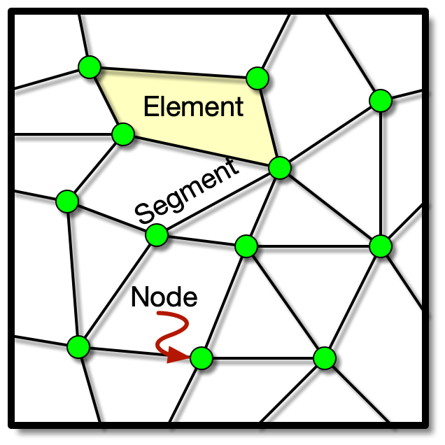
Skeletons are composed of triangular and quadrilateral elements, as shown in Figure 2.3. These are non-overlapping polygons that completely cover the Microstructure. Skeleton elements will be converted directly into Mesh Elements when a Mesh is created.

Many Skeleton operations operate on the set of currently selected elements. Elements may be selected by the Skeleton Selection Task Page and the Skeleton Selection toolbox.

2.4.2.1. Homogeneity ... or Heterogeneity

Skeleton elements inherit their Material Properties from the pixels beneath them in the Microstructure. If the Skeleton geometry is to be a good approximation of the Microstructure geometry, then all of the pixels lying beneath an element should have the same assigned Material. The homogeneity of a Skeleton element is a measure of how well the element achieves this goal. (See Figure 2.4.)

The homogeneity is computed by finding the area of the element that overlies each category of pixel. Pixels that have different assigned Materials or belong to different “meshable” PixelGroups are in different categories. The category claiming the largest area of the element is the dominant category, and the pixels in that category are the dominant pixels. The homogeneity is defined as the ratio of the area of the dominant category to the area of the element as a whole. A completely homogeneous element has a homogeneity of 1.0. An element made up of N equal components has a homogeneity of 1/N. The Material assigned to an element is the Material of its dominant pixel category.^[2]

The homogeneity index, which can be found in the Skeleton Status pane in the Skeleton Page, is the area weighted average homogeneity of all of the Elements in a Skeleton. In other words, it is the fraction of the Skeleton's area in which the Elements dominant category matches the underlying pixel category. If Skeleton that perfectly matches the Microstructure its homogeneity index is 1.0.

	Note
	The color of the pixels in an `Image` in a `Microstructure` does not directly affect the homogeneity of the elements in a `Skeleton`. Only material assignments and group membership contribute to homogeneity. However, `Image` pixel color affects materials and groups through the pixel selection mechanisms.

Figure 2.4. Skeleton Element Homogeneity

If the three different pixel colors represent different Materials, then the triangle in the upper right is completely homogeneous (homogeneity=1.0), the central triangle is inhomogeneous (homogeneity ≈ 0.5) and the leftmost triangle is even more inhomogeneous (homogeneity ≈ 0.3).

2.4.2.2. Effective Energy

Many of the tools for modifying Skeletons, such as Anneal and Smooth, work by reducing an effective energy functional, $E$ , of the mesh. This functional assigns a number between 0 and 1 to each element. It is called an energy because of its role in the Annealing operation, where it plays the role of the energy in a statistical mechanical simulated annealing process.

The energy functional has two contributions, a homogeneity energy, $E_{\mathrm{homog.}}$ and a shape energy, $E_{\mathrm{shape}}$ . Their relative importance is controlled by a parameter α:

E=\alpha E_{\mathrm{homog.}}+(1-\alpha)E_{\mathrm{shape}}

(2.1)

When $\alpha=1$ then Skeleton modifications that use $E$ will not consider the shape of elements at all, and will result in homogeneous but badly shaped elements. When $\alpha=0$ , modifications will not consider homogeneity, and will result in well shaped but possibly inhomogeneous elements. When $0<\alpha<1$ , there will be a trade-off between shape and homogeneity.

2.4.2.2.1. Homogeneity Energy

The homogeneity energy is simply one minus the homogeneity, so that it is minimized when an element is completely homogeneous.

2.4.2.2.2. Shape Energy

Finite elements are usually better behaved (the resulting matrix equations are easier to solve) if the elements do not have sharp angles or high aspect ratios. The shape energy function returns 0 for equilateral triangular or square quadrilateral elements, and 1 for elements that are degenerate (ie, have an aspect ratio of 0 or three collinear vertices).

The explicit expression for triangular elements is

E_{\mathrm{shape}}=1-4\sqrt{3}\frac{A}{L^{2}}

(2.2)

where $A$ is the area of the element and $L^{2}$ is the sum of the squares of the lengths of its sides.

For quadrilateral elements the shape energy is found by first computing a “quality factor”, $q_{i}$ , for each corner $i$ . $q_{i}$ is the area of the parallelogram defined by the two sides of the element that converge at node $i$ , divided by the sum of the squares of the sides, and normalized so that its value is 1 for a square. It's value is always less than 1 at a corner where the two converging edges have different lengths or meet at an acute or obtuse angle, and is zero in the degenerate cases when the edges are colinear or when the length of one edge is 0. The shape energy is defined to be

E_{\mathrm{shape}}=1-[(1-\epsilon)q_{\mathrm{min}}+\epsilon q_{\mathrm{opp}}]

(2.3)

where $q_{\mathrm{min}}$ is the minimum (worst) $q_{i}$ in the element, $q_{\mathrm{opp}}$ is the $q$ at the opposite corner, and $\epsilon$ is a small number. (The $\epsilon$ term is required to prevent pathologies that occur when the shape energy has no dependence on the position of one of the nodes. $\epsilon$ is set to 10^-5 in the program, but its exact value is inconsequential.)

2.4.2.3. Illegal Elements

The nodes at the corners of an element are ordered. The perimeter of the element is traversed counterclockwise when moving from one node to the next. Any operation that breaks this ordering makes the element illegal. Elements with three collinear nodes are also illegal, as are non-convex quadrilaterals. (Such elements introduce singularities and instabilities in the finite element stiffness matrix.) Figure 2.5 illustrates how node motion may create illegal elements.

Most Skeleton tools will refuse to create illegal elements. The one exception is the Move Node toolbox, which allows the user to move nodes by hand. Sometimes it may be necessary to temporarily make an illegal element while manually moving a bunch of nodes.

Figure 2.5. Creating Illegal Elements

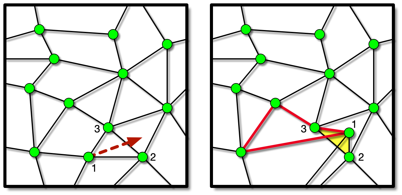
Before and after pictures of illegal elements.

Moving the node in the left hand figure results in two illegal elements in the right hand figure. The shaded triangle is illegal because its nodes (numbered 1,2,3) are out of order. The highlighted quadrilateral is illegal because it is not convex.

2.4.3. Nodes

The nodes of a Skeleton element are the corners of the element, as shown in Figure 2.3. Unlike real finite elements, Skeleton elements may not have nodes along their edges or in their interiors.

Many Skeleton operations operate on the set of currently selected nodes. Nodes may be selected by the Skeleton Selection Task Page and the Skeleton Selection toolbox.

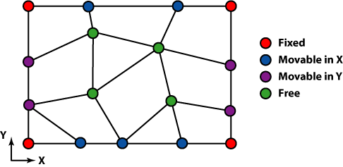
Node Mobility. Nodes may be moved when a Skeleton is modified. Different nodes have different degrees of mobility. The Nodes at the four corners of a Microstructure can never move. The Nodes along the edges of a Microstructure can move along the edge, but cannot move into the interior. All the interior Nodes can move freely (see Figure 2.6). In addition, any Node may be explicitly pinned to prevent it from moving at all.

Figure 2.6. Default Node Mobility

2.4.4. Segments

The segments of a Skeleton are the edges of the elements, i.e, the lines joining the nodes. (See Figure 2.3.)

Many Skeleton operations operate on the set of currently selected segments. Segments may be selected by the Skeleton Selection Task Page and the Skeleton Selection toolbox.

Homogeneity can be computed on Segments just as it can on Elements. Analogous to the definition of Element homogeneity, the homogeneity of a Segment is defined as the fraction of the length of the segment that lies above that Segment's dominant pixel type. See Figure 2.7 for a graphical representation.

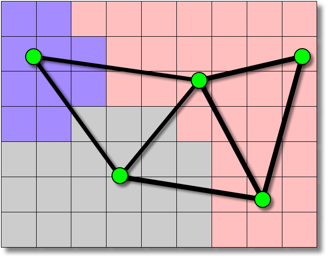
Figure 2.7. Homogeneity of a Segment

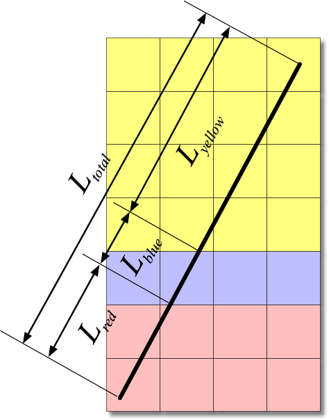
Yellow is the dominant pixel color along the segment (the heavy black line). The homogeneity of the Segment is the fractional length covered by the yellow pixels, L_yellow/L_total.

Actually, Segment homogeneity is quite a bit tricker to define than Element homogeneity. The previous discussion skipped over two subtleties which are illustrated in Figure 2.8. The first difficulty, illustrated by the vertical segment marked "A", is that the homogeneity of a segment that is part of two Elements can depend on which element is being considered. From the point of view of the left hand element, segment A is about 60% blue and 40% yellow, with the transition from blue to yellow marked by the red circle. From the point of view of the right hand element, it's about 80% yellow and 20% red, with the transition at the green circle. Because OOF2 attempts to put element edges on pixel boundaries, this sort of situation can occur quite often. OOF2 uses the correct one-sided homogeneity where it's clear which side to use, and averages the two values when it's not. The Skeleton Info Toolbox in the Graphics window reports both homogeneities when there are two distinct values.

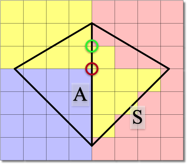
Figure 2.8. Segment Homogeneity Subtleties

The second subtlety illustrated in Figure 2.8 is what happens when a Segment lies along a diagonal pixel boundary, like the one marked "S". Again, because OOF2 puts Segments on pixel boundaries, this is a common occurence. If you were traversing this Segment looking for transition points in order to subdivide it (see Refine) you would not want to consider any of the intersections to be transition points — they are just artifacts of the pixelization of the image. This Segment should be considered to be entirely homogeneous, although whether it's yellow or red depends on which side of the segment you're interested in. OOF2 detects stairstepped pixel boundaries like this and takes them into account when computing Segment homogeneity.

2.4.5. Groups

The components of a Skeleton — elements, nodes, and segments — may be placed into named groups. These groups form a convenient way to save and recover sets of selected objects. Groups are created and manipulated by the Skeleton Selection Task Page.

2.4.6. Boundaries

Skeleton boundaries define the places where boundary conditions will be applied when solving equations on a Mesh. The Mesh inherits its boundaries from its Skeleton. There is no way to create boundaries in a Mesh directly. Boundaries may coincide with the perimeter of the Skeleton, but there is no requirement that they do so.

Boundaries are created and manipulated by the Skeleton Boundaries task page.

2.4.6.1. Edge Boundaries

Edge boundaries are composed of directed sets of conjoined segments. Each Skeleton automatically contains edge boundaries named top, bottom, left, and right. Dirichlet, Neumann, and Floating boundary conditions may be applied at edge boundaries.

2.4.6.2. Point Boundaries

Point boundaries consist of sets of nodes. Each Skeleton automatically contains point boundaries named topleft, topright, bottomleft, and bottomright. Dirichlet, Floating, and Generalized Force boundary conditions may be applied at point boundaries.

^[2] This assignment can be overridden by OOF.ElementGroup.Assign_Material.


2.3. Materials		2.5. Meshes and SubProblems