µMAG Standard Problem #4 results

Disclaimer

Solution directory

• Comparisons
• G. Albuquerque, J. Miltat and A. Thiaville
• R. D. McMichael, M. J. Donahue, D. G. Porter, and J. Eicke
• Liliana Buda, Lucian Prejbeanu, Ursula Ebels and Kamel Ounadjela
• E. Martinez, L. Torres and L. Lopez-Diaz
• José L. Martins and Tania Rocha
• P.E. Roy and P. Svedlindh
• Massimiliano d’Aquino, Claudio Serpico, and Giovanni Miano
• Dmitri Berkov
• M. J. Donahue and D. G. Porter
• Rasmus Bjørk, E. B. Poulsen and A. R. Insinga

Submitted Solution: E. Martinez, L. Torres and L. Lopez-Diaz

Date:

December 12, 2000.

From:

E. Martinez, L. Torres and L. Lopez-Diaz
Departamento de Fisica Aplicada, Universidad de Salamanca,
Plaza de la Merced s/n 37008, Spain

Contact:

Luis Torres

Our group at Salamanca, Spain, has performed simulations on the µMAG standard problem #4. The results are very close to those recently submitted by Albuquerque and McMichael groups.

A finite difference scheme in 2D (one cell across the thickness of the sample) with 3D spins was used. The exchange energy is computed by the four-neighbor dot product representation. The demagnetizing field is calculated by fast Fourier transform techniques using zero padding, and magnetostatic energy was computed under assumption that the magnetization was uniform within each cell and it is allowed to rotate in 3D. The demagnetizing tensor is calculated using Newell's expressions (average over the volume of each cell) particularized to 2D. Three sizes for the cell were tested: 5 nm, 3.125 nm, and 2.5 nm cells. Our code was previously used successfully to resolve the µMAG standard problem #2 [J. Appl. Phys. 85 (8), 5813, (1999)].

The Landau-Lifshitz equation was resolved using the Euler's method with different time steps in the range 3-15 fs (femtoseconds). A time step of 3.14 fs was used to calculate the results shown below. In the case of 2.5 nm cells, because of the simple Euler's method utilised, time steps less than 5nm were necessary for obtaining an adequate convergence of the solution. Larger time steps produced oscillating solutions.

Results:

• Field 1

  
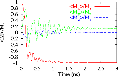
  The temporal evolution of the magnetization components spatially averaged over the sample is represented using 2.5 nm cell size and time step of 3.14 fs for the field applied 170° from the x-axis.

  
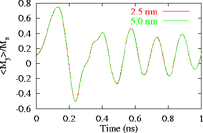
  Comparison of M_y vs. t data calculated with 2.5 nm cells and 5 nm cells. In this case, the results are insensitive to the mesh (No difference is appreciated in the figure).

  
  An image of the magnetization when M_x first crosses zero.

• Field 2

  
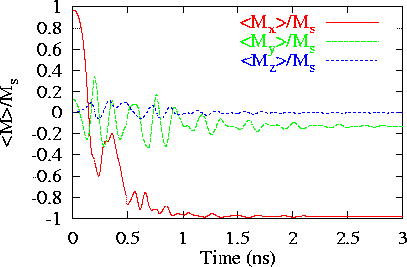
  M vs. t for the second part of the problem, with the field applied 190° from the x-axis (Field 2), with 2.5 nm cell size and time step of 3.14 fs.

  
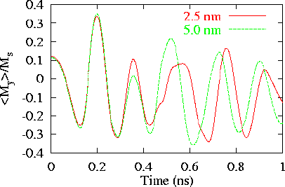
  Comparison of M_y vs. t data calculated with 2.5 nm cells and 5 nm cells. These results show dependence on the mesh size. The differences increase with time.

  
  Finally, an image of the magnetization when M_x first crosses zero.

Raw Data:

• Field 1: Time series for 2.5 nm mesh, Time series for 5.0 nm mesh, and Vector data at < M_x > = 0.
• Field 2: Time series for 2.5 nm mesh, Time series for 5.0 nm mesh, and Vector data at < M_x > = 0.

Time series data contain 4 columns: time (ns), M_x/M_s, M_y/M_s, M_z/M_s, and vector data is in omf format.