µMAG Standard Problem #2 Results

Disclaimer

Solution directory

• Comparisons
• B Streibl, T Schrefl and J Fidler
• R. D. McMichael, M. J. Donahue, D. G. Porter, and J. Eicke
• L. L. Diaz L. Torres, J. I. Iniguez and O. Alejos
• M. J. Donahue, D. G. Porter, R. D. McMichael, and J. Eicke
• Rasmus Bjørk, E. B. Poulsen and A. R. Insinga

Summary Plots, µMAG Problem #2

Coercivity for fields applied along the (111) direction as a function of d/l_ex.

Submitted Solution

Solution to standard problem #2

From:   B Streibl, T Schrefl and J Fidler
             Institute of Applied and Technical Physics
             Vienna University of Technology
             Wiedner Hauptstr. 8-10
             A-1040 Vienna, Austria

Contact: T Schrefl
URL:      http://magnet.atp.tuwien.ac.at/

Reference: B. Streibl, T. Schrefl and J. Fidler, J. Appl. Phys, v. 85, pp 5819-5821 (1999).

We studied standard problem #2 using a 3D-finite element simulation based on the solution of the Gilbert equation. Asymptotic boundary conditions were imposed in order to compute demagnetizing fields. The direction cosines of the magnetization and the magnetic scalar potential were interpolated with piecewise linear and quadratic polynomials on hexahedral finite elements, respectively. The finest mesh used for the calculations contains 500 elements within the magnetic thin film and 4200 in the exterior space. The values of  Permalloy were assumed for the magnetization and the exchange constant, so that the exchange length l_ex becomes 5 nm.
A Gilbert-damping parameter (alpha=1) was used to drive the system towards equilibrium. For more details on the calculation method we refer to our forthcoming paper "Dynamic FE-simulation of mumag standard problem #2" which will be presented at the 43rd annual conference on Magnetism & Magnetic Materials in Miami, November 9-12, 1998 (session FZ-05).

1. For the coercive field and the remanence magnetization we find for varying particle extensions and the external field applied parallel to the [111]-direction:


 

d/lex	Mrx/Ms	Mry/Ms	Mrz/Ms	Hc/Ms
1	0.999	0.029	-0.004	-0.056
5	0.999	0.006	0.000	-0.056
10	0.998	0.020	0.000	-0.054
20	0.973	0.081	0.000	-0.050
30	0.963	0.078	0.000	-0.046

(The coordinate axis are oriented as proposed in the specification of the standard problem)
 

2. Images:
• Demagnetizing curves obtained with the field parallel to the [111]-direction for particles with width
• d=10*l_ex
• d=20*l_ex
• d=30*l_ex

(l_ex denotes the exchange length)

• Magnetization configurations appearing during demagnetization of a particle with d=20*l_ex in a [111]-field


(M denotes the component of the magnetization parallel to the field)

• Transient states during irreversible switching in a [100]-field for particles with width
• d=10*l_ex
• d=20*l_ex
• d=30*l_ex

Submitted Solution

Contact: Bob McMichael

Reference: R. D. McMichael, M. J. Donahue, D. G. Porter and Jason Eicke, J. Appl. Phys, v. 85, pp 5816-5818 (1999).

We used the OOMMF public code to compute solutions to standard problem #2. The mesh was a 2D square grid with 3D spins interacting through an 8-neighbor exchange representation and magnetostatic fields. Computations were done for a number of mesh sizes, using up to 12500 cells, using energy minimization (precession neglected). We obtained similar results for two methods of calculating the magnetostatic fields, the constant magnetization method, and the constant charge method.

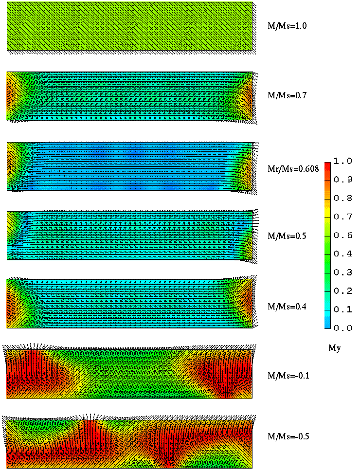
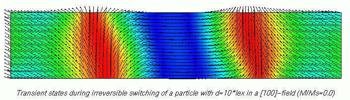
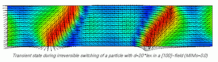
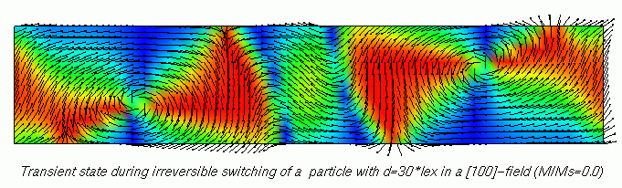
We find three types of critical fields, end domain switching, end domain propagation, and vortex formation, depending on the value of d/l_ex. These critical field values, extrapolated to zero cell size, are listed below in terms of H_c/M_s with an uncertainty of plus/minus 0.0014, corresponding to the field step size. The remanent magnetization values, calculated by relaxing from saturation in the (111) direction are also listed.

	Hcrit/Ms			Remanence
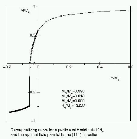
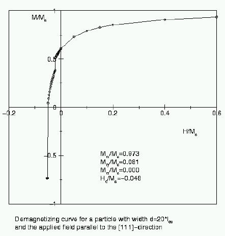
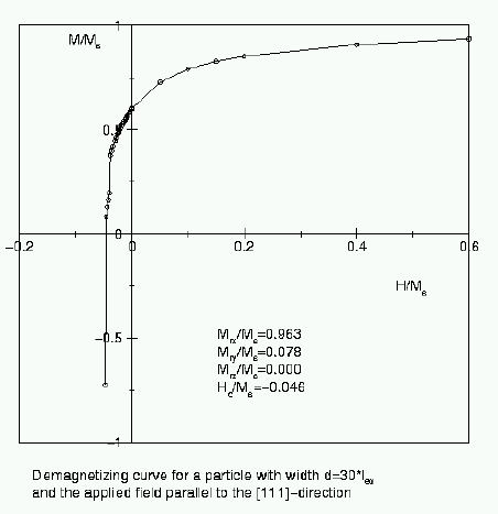
d/lex	end propagation	end switch	vortex formation	Mx/Ms	My/Ms	Mz/Ms
3.16	0.0600			1.0000	0.0007	0.0000
10	0.0586	0.0007		0.9959	0 .0376	-0.0000
14	0.0558	0.0145		0.9783	0.0822	0.0000
17.8	0.0531	0.0278		0.9711	0.0851	0.0000
23	0.0503	0.0393		0.9657	0.0823	0.0000
27	0.0489	0.0448		0.9631	0.0792	0.0000
31.6		0.0517		0.9609	0.0760	0.0000
35		0.0553		0.9595	0.0739	0.0000
40			0.0532	0.9577	0.0710	0.0000
56			0.0408	0.9527	0.0638	0.0000
75			0.0200	0.9478	0.0572	0.0003

Images

• Plot of critical fields
• Calculated domain pattern images .

Submitted Solution

Contact: Luis Lopez Diaz

Reference: L. Lopez-Diaz, O. Alejos, L. Torres and J. I. Iniguez J. Appl. Phys, v. 85, pp 5813-5815 (1999).

d/lex	Hc/Ms	M[111]	Mrx	Mry
0.8	0.0631	0.5773740	1.00000	7.00000E-05
1.0	0.0612	0.5773501	1.00000	7.00000E-05
2.0	0.0594	0.5773470	0.999996	4.27499E-05
3.0	0.0596	0.5773384	0.999981	-1.24466E-07
4.0	0.0594	0.5773172	0.999942	4.14687E-05
5.0	0.0592	0.5772781	0.999876	3.95000E-05
6.0	0.0585	0.5772195	0.999777	-7.30804E-08
7.0	0.0583	0.5771367	0.999596	8.22480E-08
8.0	0.0580	0.5770244	0.999439	3.25319E-05
9.0	0.0576	0.5769020	0.999191	6.88017E-05
10.0	0.0573	0.5956421	0.996272	3.54161E-02
11.0	0.0568	0.6069226	0.989998	6.12417E-02
12.0	0.0565	0.6106740	0.985207	7.25276E-02
13.0	0.0560	0.6120005	0.981448	7.85834E-02
14.0	0.0556	0.6122172	0.978436	8.19699E-02
15.0	0.0549	0.6118625	0.975986	8.38084E-02
16.0	0.0541	0.6112075	0.973947	8.47102E-02
17.0	0.0534	0.6103936
18.0	0.0529	0.6095005	0.970768	8.49321E-02
20.0	0.0518	0.6076426

Submitted Solution

Contact: Mike Donahue (URL: http://math.nist.gov/mcsd/Staff/MDonahue/)

Reference: J. Appl. Phys, .v 87, pp. 5520-5522 (2000).

An examination of the coercive fields from first three submissions (Streibl et al., McMichael et al., Diaz et al.) reveals discrepancies in the small particle limit (d/l_ex near 0). In this range the magnetization is nearly uniform, so we performed a 3D Stoner-Wohlfarth analysis, and found the theoretical value for the coercive field to be H_c/M_s = 0.05707. This result is in close agreement with the Streibl submission, but is removed from our first calculation (McMichael), which was based on version 1.0 of the OOMMF public code.

In the uniformly magnetized setting, only magnetostatic energies are active. We therefore examined the demagnetization (self-magnetostatic) energy calculated by OOMMF as a function of calculation cell size for the uniformly magnetized particle. It is observed that the sampled H_demag model used in OOMMF 1.0 for demagnetization energy calculations is inaccurate in this case.

The magnetostatic energy between two uniformly magnetized rectangular prisms can be evaluated analytically (A. J. Newell, W. Williams, and D. J. Dunlop, J. Geophysical Research, 98, 9551 (1993)). From the standpoint of calculating demagnetization energy, these formulae can be viewed as providing a value for H_demag that has been averaged over the calculation cell. The averaged H_demag model is also completely accurate for uniformly magnetized particles (as seen in the aforementioned graph).

In the small particle range, the accuracy of the averaged H_demag formulae allowed us to use calculation cells that were large compared to d. We could then run simulations at smaller values of d/l_ex than we had in our earlier submission. We discovered, however, that numerical errors in the calculation of the exchange energy produced an artificial stiffening of the simulation. We were able to reduce this problem by replacing our base exchange energy term 1-m_i·m_k (m_i and m_k are neighboring spins) with an expression of the form m_i·(m_i - m_k).

These changes have been incorporated into version 1.1 of OOMMF, which was used to produce this submission. From the summary coercive field plot above, we see that OOMMF 1.1 closely tracks the Streibl results, and agrees with the theoretical result for the infinitely small particle case.

It is worth noting that the switching field H_s (the field at which the first irreversible change in magnetization occurs) is somewhat larger that the coercive field H_c (the field at which H_applied·M =0) for d/l_ex<15, as illustrated by this graph. We found that the theoretical value for the switching field in the small particle limit was H_s/M_s = 0.05714, also slightly higher than the coercive field.

The table below presents our results using OOMMF 1.1 with the changes outlined above. H_c is the coercive field, H_s is the switching field, M_x and M_y are the average x and y magnetizations at remanence. MaxAngle/run is the largest angle between neighboring spins (i.e., calculation elements) that occurred throughout the simulation, including non-equilibrium states; this is an indication of the ability of the sample mesh to represent the variation in the magnetization. The uncertainty in the field values H_c and H_s due to the applied field step size is less than ±0.0000138 M_s. In particular, the results at d/l_ex=0.125 agree to within this precision with the theoretical results for an infinitely small particle.

d/lex	Cellsize/ lex	Hc/Ms	Hs/Ms	Mx/Ms	My/Ms	MaxAngle/ run (deg)
30	0.60	0.04594	0.04594	0.9627	0.0756	13.4
29	0.58	0.04630	0.04630	0.9632	0.0763	12.8
28	0.56	0.04666	0.04666	0.9638	0.0769	12.2
27	0.54	0.04704	0.04704	0.9644	0.0776	11.6
26	0.52	0.04740	0.04740	0.9650	0.0783	11.0
25	0.50	0.04779	0.04779	0.9657	0.0790	10.4
24	0.48	0.04817	0.04817	0.9664	0.0797	9.75
23	0.46	0.04859	0.04859	0.9672	0.0803	9.16
22	0.44	0.04903	0.04903	0.9680	0.0809	8.57
21	0.42	0.04947	0.04947	0.9690	0.0814	7.98
20	0.40	0.04991	0.04991	0.9701	0.0819	7.41
19	0.38	0.05041	0.05041	0.9713	0.0822	6.85
18	0.36	0.05090	0.05090	0.9727	0.0822	6.31
17	0.34	0.05145	0.05145	0.9743	0.0819	5.77
16	0.32	0.05200	0.05200	0.9762	0.0811	5.25
15	0.30	0.05258	0.05261	0.9784	0.0795	4.73
14	0.56	0.05309	0.05324	0.9812	0.0765	8.4
13	0.52	0.05352	0.05388	0.9845	0.0716	7.5
12	0.48	0.05389	0.05449	0.9886	0.0631	6.8
11	0.44	0.05423	0.05506	0.9938	0.0463	6.1
10	0.40	0.05454	0.05562	0.9989	0.0000	5.1
9	0.45	0.05480	0.05614	0.9992	0.0000	4.0
8	0.40	0.05515	0.05661	0.9995	0.0000	4.0
7	0.35	0.05546	0.05702	0.9996	0.0000	3.2
6	0.30	0.05579	0.05730	0.9998	0.0000	2.4
5	0.25	0.05612	0.05741	0.9999	0.0000	1.8
4	0.20	0.05646	0.05735	0.9999	0.0000	1.2
3	0.15	0.05674	0.05724	1.0000	0.0000	0.696
2	0.10	0.05694	0.05716	1.0000	0.0000	0.314
1	0.05	0.05704	0.05716	1.0000	0.0000	0.079
0.75	0.15	0.05705	0.05713	1.0000	0.0000	0.182
0.50	0.10	0.05706	0.05713	1.0000	0.0000	0.0813
0.25	0.05	0.05707	0.05713	1.0000	0.0000	0.0204
0.125	0.03	0.05707	0.05713	1.0000	0.0000	0.0063
Theory	n/a	0.05707	0.05714	1.0000	0.0000	n/a

Submitted Solution

Contact: Rasmus Bjørk (URL: http://www.magtense.org)

Reference: J. Magn. Magn. Mater., .v 535, pp. 168057 (2021), DOI: https://doi.org/10.1016/j.jmmm.2021.168057

We used the MagTense open source micromagnetic simulation framework to compute solutions to standard problem #2. The mesh was a 3D square grid with 3D spins. A Cartesian mesh with 100x20x3 rectangular cuboid tiles in the x-, y- and z-directions respectively were utilized. The hysteresis loop for each individual value of d/l_ex was computed by starting with an applied field of 0.08 H/M_s and then decreasing the field in 4000 steps to a value of -0.08 H/M_s. The micromagnetic damping parameter is taken to be 4000, close to the value for mumag standard problem 4, and the precession parameter is taken to be 0. The demagnetization field was calculated using an analytical approach, assuming only a constant magnetization within each grid cell. The exchange field was calculated using a finite difference approach.

We find the results as tabulated below

d/lex	Hc/Ms	Mrx	Mry
3.00	0.05705	1.000000	8.69376e-4
4.93	0.05586	0.999885	3.55424e-4
6.86	0.05507	0.999667	2.90060e-4
8.79	0.05441	0.999290	7.83946e-4
10.71	0.05378	0.996211	3.40159e-2
12.64	0.05310	0.986592	6.72743e-2
14.57	0.05229	0.980252	7.71206e-2
16.50	0.05133	0.975886	8.05364e-2
18.43	0.05032	0.972714	8.13575e-2
20.36	0.04938	0.970298	8.09996e-2
22.29	0.04851	0.968385	8.00821e-2
24.21	0.04772	0.966817	7.89040e-2
26.14	0.04698	0.965493	7.76162e-2
28.07	0.04627	0.964346	7.62986e-2
30.00	0.04558	0.963332	7.49929e-2