 FiPy
FiPyexamples.phase.binaryCoupled
Simultaneously solve a phase-field evolution and solute diffusion problem in one-dimension.
It is straightforward to extend a phase field model to include binary alloys.
As in examples.phase.simple, we will examine a 1D problem
>>> from fipy import CellVariable, Variable, Grid1D, TransientTerm, DiffusionTerm, ImplicitSourceTerm, LinearLUSolver, Viewer
>>> from fipy.tools import numerix
>>> nx = 400
>>> dx = 5e-6 # cm
>>> L = nx * dx
>>> mesh = Grid1D(dx=dx, nx=nx)
The Helmholtz free energy functional can be written as the integral [1] [3] [24]

over the volume  as a function of phase
  [1]
[1]
>>> phase = CellVariable(name="phase", mesh=mesh, hasOld=1)
composition 
>>> C = CellVariable(name="composition", mesh=mesh, hasOld=1)
and temperature  [2]
[2]
>>> T = Variable(name="temperature")
Frequently, the gradient energy term in concentration is ignored and we can derive governing equations
(1)
for phase and
(2)
for solute.
The free energy density  can be constructed in many
different ways. One approach is to construct free energy densities for
each of the pure components, as functions of phase, e.g.
can be constructed in many
different ways. One approach is to construct free energy densities for
each of the pure components, as functions of phase, e.g.

where  ,
,  ,
,  , and
, and  are the free energy densities of the pure components. There are a
variety of choices for the interpolation function
are the free energy densities of the pure components. There are a
variety of choices for the interpolation function  and the
barrier function
and the
barrier function  ,
,
such as those shown in examples.phase.simple
>>> def p(phi):
...     return phi**3 * (6 * phi**2 - 15 * phi + 10)
>>> def g(phi):
...     return (phi * (1 - phi))**2
The desired thermodynamic model can then be applied to obtain
, such as for a regular solution,
![f(\phi, C, T) &= (1 - C) f_A(\phi, T) + C f_B(\phi, T) \\
&\qquad + R T \left[
(1 - C) \ln (1 - C) + C \ln C
\right]
+ C (1 - C) \left[
\Omega_S p(\phi)
+ \Omega_L \left( 1 - p(\phi) \right)
\right]](../../../_images/math/7c442caa4856615899db5afa637cc5fbeb949821.svg)
where
>>> R = 8.314 # J / (mol K)
is the gas constant and  and
and  are the
regular solution interaction parameters for solid and liquid.
are the
regular solution interaction parameters for solid and liquid.
Another approach is useful when the free energy densities  and
and  of the alloy in the solid and liquid phases are
known. This might be the case when the two different phases have
different thermodynamic models or when one or both is obtained from a
Calphad code. In this case, we can construct
of the alloy in the solid and liquid phases are
known. This might be the case when the two different phases have
different thermodynamic models or when one or both is obtained from a
Calphad code. In this case, we can construct
![f(\phi, C, T) = p(\phi) f^S(C,T)
+ \left(1 - p(\phi)\right) f^L(C, T)
+ \left[
(1-C) \frac{W_A}{2} + C \frac{W_B}{2}
\right] g(\phi).](../../../_images/math/c94056b6d8e8614f5d03c4c07faf09116daf1a8c.svg)
When the thermodynamic models are the same in both phases, both approaches should yield the same result.
We choose the first approach and make the simplifying assumptions of an ideal solution and that

and likewise for component  .
.
>>> LA = 2350. # J / cm**3
>>> LB = 1728. # J / cm**3
>>> TmA = 1728. # K
>>> TmB = 1358. # K
>>> enthalpyA = LA * (T - TmA) / TmA
>>> enthalpyB = LB * (T - TmB) / TmB
This relates the difference between the free energy densities of the
pure solid and pure liquid phases to the latent heat  and the
pure component melting point
and the
pure component melting point  , such that

With these assumptions
(3)
and
(4)¶![\frac{\partial f}{\partial C}
&= \left[f_B(\phi, T) + \frac{R T}{V_m} \ln C\right]
- \left[f_A(\phi, T) + \frac{R T}{V_m} \ln (1-C) \right] \nonumber \\
&= \left[\mu_B(\phi, C, T) - \mu_A(\phi, C, T) \right] / V_m](../../../_images/math/975f9cebd479194d120b7943d52a391e024714f0.svg)
where  and
and  are the classical chemical potentials
for the binary species.
are the classical chemical potentials
for the binary species.  and
and  are the
partial derivatives of of
are the
partial derivatives of of  and
and  with respect to
>>> def pPrime(phi):
...     return 30. * g(phi)
>>> def gPrime(phi):
...     return 2. * phi * (1 - phi) * (1 - 2 * phi)
 is the molar volume, which we take to be independent of
concentration and phase
is the molar volume, which we take to be independent of
concentration and phase
>>> Vm = 7.42 # cm**3 / mol
On comparison with examples.phase.simple, we can see that the
present form of the phase field equation is identical to the one found
earlier, with the source now composed of the concentration-weighted average
of the source for either pure component. We let the pure component barriers
equal the previous value
>>> deltaA = deltaB = 1.5 * dx
>>> sigmaA = 3.7e-5 # J / cm**2
>>> sigmaB = 2.9e-5 # J / cm**2
>>> betaA = 0.33 # cm / (K s)
>>> betaB = 0.39 # cm / (K s)
>>> kappaA = 6 * sigmaA * deltaA # J / cm
>>> kappaB = 6 * sigmaB * deltaB # J / cm
>>> WA = 6 * sigmaA / deltaA # J / cm**3
>>> WB = 6 * sigmaB / deltaB # J / cm**3
and define the averages
>>> W = (1 - C) * WA / 2. + C * WB / 2.
>>> enthalpy = (1 - C) * enthalpyA + C * enthalpyB
We can now linearize the source exactly as before
>>> mPhi = -((1 - 2 * phase) * W + 30 * phase * (1 - phase) * enthalpy)
>>> dmPhidPhi = 2 * W - 30 * (1 - 2 * phase) * enthalpy
>>> S1 = dmPhidPhi * phase * (1 - phase) + mPhi * (1 - 2 * phase)
>>> S0 = mPhi * phase * (1 - phase) - S1 * phase
Using the same gradient energy coefficient and phase field mobility
>>> kappa = (1 - C) * kappaA + C * kappaB
>>> Mphi = TmA * betaA / (6 * LA * deltaA)
we define the phase field equation
>>> phaseEq = (TransientTerm(1/Mphi, var=phase) == DiffusionTerm(coeff=kappa, var=phase)
...            + S0 + ImplicitSourceTerm(coeff=S1, var=phase))
When coding explicitly, it is typical to simply write a function to
evaluate the chemical potentials and and then
perform the finite differences necessary to calculate their gradient and
divergence, e.g.,:
def deltaChemPot(phase, C, T):
    return ((Vm * (enthalpyB * p(phase) + WA * g(phase)) + R * T * log(1 - C)) -
            (Vm * (enthalpyA * p(phase) + WA * g(phase)) + R * T * log(C)))

for j in range(faces):
    flux[j] = ((Mc[j+.5] + Mc[j-.5]) / 2) \
      * (deltaChemPot(phase[j+.5], C[j+.5], T) \
        - deltaChemPot(phase[j-.5], C[j-.5], T)) / dx

for j in range(cells):
    diffusion = (flux[j+.5] - flux[j-.5]) / dx
where we neglect the details of the outer boundaries (j = 0 and j = N)
or exactly how to translate j+.5 or j-.5 into an array index,
much less the complexities of higher dimensions. FiPy can handle all of
these issues automatically, so we could just write:
chemPotA = Vm * (enthalpyA * p(phase) + WA * g(phase)) + R * T * log(C)
chemPotB = Vm * (enthalpyB * p(phase) + WB * g(phase)) + R * T * log(1-C)
flux = Mc * (chemPotB - chemPotA).faceGrad
eq = TransientTerm() == flux.divergence
Although the second syntax would essentially work as written, such an explicit implementation would be very slow. In order to take advantage of FiPy’s implicit solvers, it is necessary to reduce Eq. (2) to the canonical form of Eq. (2), hence we must expand Eq. (4) as
![\frac{\partial f}{\partial C}
= \left[
\frac{L_B\left(T - T_M^B\right)}{T_M^B}
- \frac{L_A\left(T - T_M^A\right)}{T_M^A}
\right] p(\phi)
+ \frac{R T}{V_m} \left[\ln C - \ln (1-C)\right]
+ \frac{W_B - W_A}{2} g(\phi)](../../../_images/math/1e79bbad149a91196f46dedcbd150a521534b636.svg)
In either bulk phase,  , so
we can then reduce Eq. (2) to
, so
we can then reduce Eq. (2) to
(5)¶![\frac{\partial C}{\partial t}
&= \nabla\cdot\left( M_C \nabla \left\{
\frac{R T}{V_m} \left[\ln C - \ln (1-C)\right]
\right\}
\right) \nonumber \\
&= \nabla\cdot\left[
\frac{M_C R T}{C (1-C) V_m} \nabla C
\right]](../../../_images/math/df6fb791604764af378ca2d1cbe30e71700c83b0.svg)
and, by comparison with Fick’s second law
![\frac{\partial C}{\partial t}
= \nabla\cdot\left[D \nabla C\right],](../../../_images/math/a0f646014de1837a0f5a76db701948f5e1d65eea.svg)
we can associate the mobility  with the intrinsic diffusivity
  by
by
 and write Eq. (2) as
(6)¶![\frac{\partial C}{\partial t}
&= \nabla\cdot\left( D_C \nabla C \right) \nonumber \\
&\qquad + \nabla\cdot\left(
\frac{D_C C (1 - C) V_m}{R T}
\left\{
\left[
\frac{L_B\left(T - T_M^B\right)}{T_M^B}
- \frac{L_A\left(T - T_M^A\right)}{T_M^A}
\right] \nabla p(\phi)
+ \frac{W_B - W_A}{2} \nabla g(\phi)
\right\}
\right). \\
&= \nabla\cdot\left( D_C \nabla C \right) \nonumber \\
&\qquad + \nabla\cdot\left(
\frac{D_C C (1 - C) V_m}{R T}
\left\{
\left[
\frac{L_B\left(T - T_M^B\right)}{T_M^B}
- \frac{L_A\left(T - T_M^A\right)}{T_M^A}
\right] p'(\phi)
+ \frac{W_B - W_A}{2} g'(\phi)
\right\} \nabla \phi
\right).](../../../_images/math/4351f58276b4f68d494b42835d6c28d82e2465eb.svg)
The first term is clearly a DiffusionTerm in . The second is a
DiffusionTerm in with a diffusion coefficient
![D_{\phi}(C, \phi) =
\frac{D_C C (1 - C) V_m}{R T}
\left\{
\left[
\frac{L_B\left(T - T_M^B\right)}{T_M^B}
- \frac{L_A\left(T - T_M^A\right)}{T_M^A}
\right] p'(\phi)
+ \frac{W_B - W_A}{2} g'(\phi)
\right\},](../../../_images/math/07a93ba8851970bac97f20210361303a78c50ce2.svg)
such that

or
>>> Dl = Variable(value=1e-5) # cm**2 / s
>>> Ds = Variable(value=1e-9) # cm**2 / s
>>> Dc = (Ds - Dl) * phase.arithmeticFaceValue + Dl
>>> Dphi = ((Dc * C.harmonicFaceValue * (1 - C.harmonicFaceValue) * Vm / (R * T))
...         * ((enthalpyB - enthalpyA) * pPrime(phase.arithmeticFaceValue)
...            + 0.5 * (WB - WA) * gPrime(phase.arithmeticFaceValue)))
>>> diffusionEq = (TransientTerm(var=C)
...                == DiffusionTerm(coeff=Dc, var=C)
...                + DiffusionTerm(coeff=Dphi, var=phase))
>>> eq = phaseEq & diffusionEq
We initialize the phase field to a step function in the middle of the domain
>>> phase.setValue(1.)
>>> phase.setValue(0., where=mesh.cellCenters[0] > L/2.)
and start with a uniform composition field 
>>> C.setValue(0.5)
In equilibrium,  and
and
 and, for ideal solutions, we can
deduce the liquidus and solidus compositions as
and, for ideal solutions, we can
deduce the liquidus and solidus compositions as

>>> Cl = ((1. - numerix.exp(-enthalpyA * Vm / (R * T)))
...       / (numerix.exp(-enthalpyB * Vm / (R * T)) - numerix.exp(-enthalpyA * Vm / (R * T))))
>>> Cs = numerix.exp(-enthalpyB * Vm / (R * T)) * Cl
The phase fraction is predicted by the lever rule
>>> Cavg = C.cellVolumeAverage
>>> fraction = (Cl - Cavg) / (Cl - Cs)
For the special case of fraction = Cavg = 0.5, a little bit of algebra
reveals that the temperature that leaves the phase fraction unchanged is
given by
>>> T.setValue((LA + LB) * TmA * TmB / (LA * TmB + LB * TmA))
In this simple, binary, ideal solution case, we can derive explicit expressions for the solidus and liquidus compositions. In general, this may not be possible or practical. In that event, the root-finding facilities in SciPy can be used.
We’ll need a function to return the two conditions for equilibrium

>>> def equilibrium(C):
...     return [numerix.array(enthalpyA * Vm
...                           + R * T * numerix.log(1 - C[0])
...                           - R * T * numerix.log(1 - C[1])),
...             numerix.array(enthalpyB * Vm
...                           + R * T * numerix.log(C[0])
...                           - R * T * numerix.log(C[1]))]
and we’ll have much better luck if we also supply the Jacobian
![\left[\begin{matrix}
\frac{\partial(\mu_A^S - \mu_A^L)}{\partial C_S}
& \frac{\partial(\mu_A^S - \mu_A^L)}{\partial C_L} \\
\frac{\partial(\mu_B^S - \mu_B^L)}{\partial C_S}
& \frac{\partial(\mu_B^S - \mu_B^L)}{\partial C_L}
\end{matrix}\right]
=
R T\left[\begin{matrix}
-\frac{1}{1-C_S} & \frac{1}{1-C_L} \\
\frac{1}{C_S} & -\frac{1}{C_L}
\end{matrix}\right]](../../../_images/math/cf87ed799b98e40c31728585176e346bdade41ac.svg)
>>> def equilibriumJacobian(C):
...     return R * T * numerix.array([[-1. / (1 - C[0]), 1. / (1 - C[1])],
...                                   [ 1. / C[0],      -1. / C[1]]])
>>> try:
...     from scipy.optimize import fsolve
...     CsRoot, ClRoot = fsolve(func=equilibrium, x0=[0.5, 0.5],
...                             fprime=equilibriumJacobian)
... except ImportError:
...     ClRoot = CsRoot = 0
...     print("The SciPy library is not available to calculate the solidus and ... liquidus concentrations")
>>> print(Cl.allclose(ClRoot))
1
>>> print(Cs.allclose(CsRoot))
1
We plot the result against the sharp interface solution
>>> sharp = CellVariable(name="sharp", mesh=mesh)
>>> x = mesh.cellCenters[0]
>>> sharp.setValue(Cs, where=x < L * fraction)
>>> sharp.setValue(Cl, where=x >= L * fraction)
>>> if __name__ == '__main__':
...     viewer = Viewer(vars=(phase, C, sharp),
...                     datamin=0., datamax=1.)
...     viewer.plot()
Because the phase field interface will not move, and because we’ve seen in earlier examples that the diffusion problem is unconditionally stable, we need take only one very large timestep to reach equilibrium
>>> dt = 1.e5
Because the phase field equation is coupled to the composition through
enthalpy and W and the diffusion equation is coupled to the phase
field through phaseTransformationVelocity, it is necessary sweep this
non-linear problem to convergence. We use the “residual” of the equations
(a measure of how well they think they have solved the given set of linear
equations) as a test for how long to sweep.
We now use the “sweep()” method instead of
“solve()” because we require the residual.
>>> solver = LinearLUSolver(tolerance=1e-10)
>>> phase.updateOld()
>>> C.updateOld()
>>> res = 1.
>>> initialRes = None
>>> sweep = 0
>>> while res > 1e-4 and sweep < 20:
...     res = eq.sweep(dt=dt, solver=solver)
...     if initialRes is None:
...         initialRes = res
...     res = res / initialRes
...     sweep += 1
>>> from fipy import input
>>> if __name__ == '__main__':
...     viewer.plot()
...     input("Stationary phase field. Press <return> to proceed...")
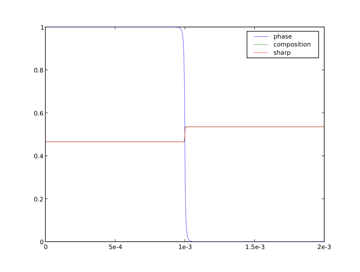
We verify that the bulk phases have shifted to the predicted solidus and liquidus compositions
>>> X = mesh.faceCenters[0]
>>> print(Cs.allclose(C.faceValue[X.value==0], atol=1e-2))
True
>>> print(Cl.allclose(C.faceValue[X.value==L], atol=1e-2))
True
and that the phase fraction remains unchanged
>>> print(fraction.allclose(phase.cellVolumeAverage, atol=2e-4))
1
while conserving mass overall
>>> print(Cavg.allclose(0.5, atol=1e-8))
1
We now quench by ten degrees
>>> T.setValue(T() - 10.) # K
>>> sharp.setValue(Cs, where=x < L * fraction)
>>> sharp.setValue(Cl, where=x >= L * fraction)
Because this lower temperature will induce the phase interface to move (solidify), we will need to take much smaller timesteps (the time scales of diffusion and of phase transformation compete with each other).
The CFL limit requires that no interface should advect more than one grid spacing in a timestep. We can get a rough idea for the maximum timestep we can take by looking at the velocity of convection induced by phase transformation in Eq. (6) (even though there is no explicit convection in the coupled form used for this example, the principle remains the same). If we assume that the phase changes from 1 to 0 in a single grid spacing, that the diffusivity is Dl at the interface, and that the term due to the difference in barrier heights is negligible:
![\vec{u}_\phi &= \frac{D_\phi}{C} \nabla \phi
\\
&\approx
\frac{Dl \frac{1}{2} V_m}{R T}
\left[
\frac{L_B\left(T - T_M^B\right)}{T_M^B}
- \frac{L_A\left(T - T_M^A\right)}{T_M^A}
\right] \frac{1}{\Delta x}
\\
&\approx
\frac{Dl \frac{1}{2} V_m}{R T}
\left(L_B + L_A\right) \frac{T_M^A - T_M^B}{T_M^A + T_M^B}
\frac{1}{\Delta x}
\\
&\approx \unit{0.28}{\centi\meter\per\second}](../../../_images/math/e03b0179773dd4853ec4c33f0a19f302481f78fa.svg)
To get a  , we need a
time step of about
, we need a
time step of about  .
.
>>> dt = 1.e-5
>>> if __name__ == '__main__':
...     timesteps = 100
... else:
...     timesteps = 10
>>> from builtins import range
>>> for i in range(timesteps):
...     phase.updateOld()
...     C.updateOld()
...     res = 1e+10
...     sweep = 0
...     while res > 1e-3 and sweep < 20:
...         res = eq.sweep(dt=dt, solver=solver)
...         sweep += 1
...     if __name__ == '__main__':
...         viewer.plot()
>>> from fipy import input
>>> if __name__ == '__main__':
...     input("Moving phase field. Press <return> to proceed...")
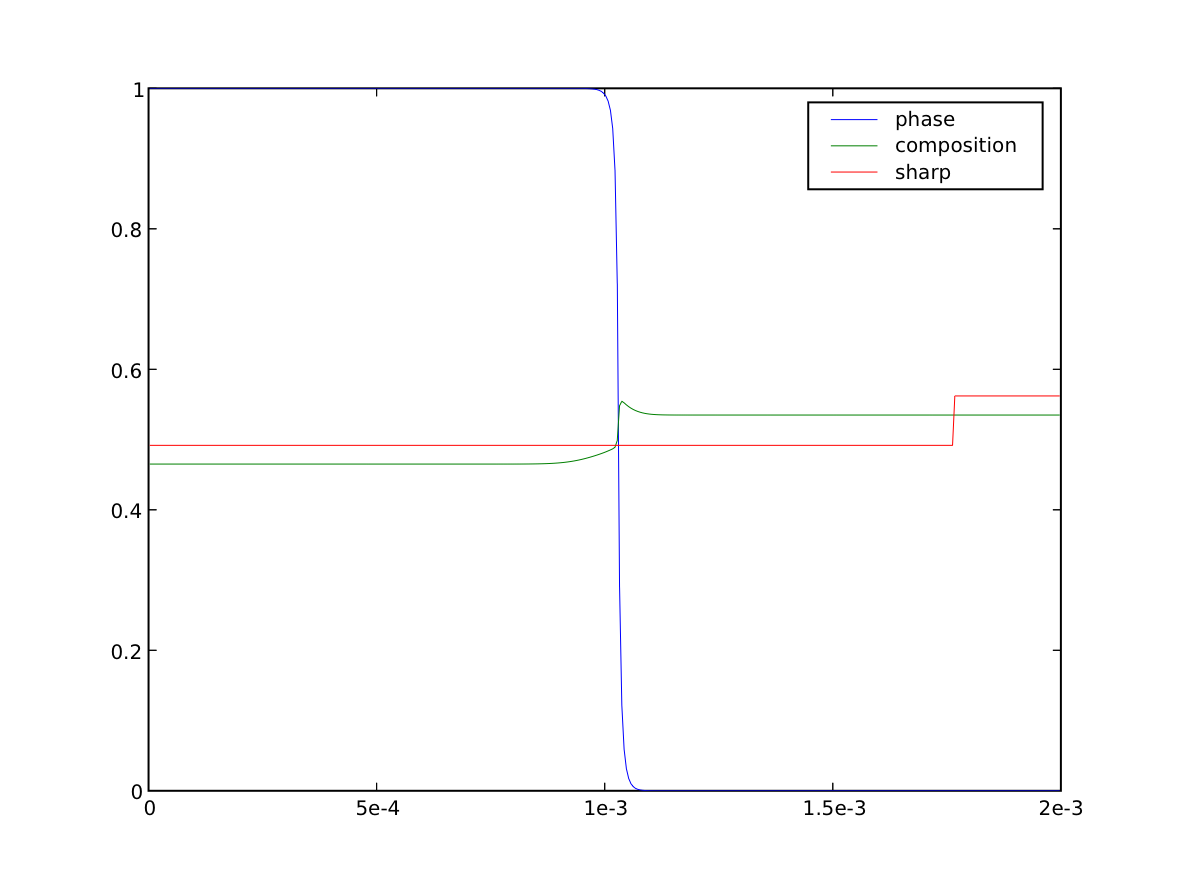
We see that the composition on either side of the interface approach the sharp-interface solidus and liquidus, but it will take a great many more timesteps to reach equilibrium. If we waited sufficiently long, we could again verify the final concentrations and phase fraction against the expected values.
Footnotes