examples.phase.simple¶

Solve a phase-field (Allen-Cahn) problem in one-dimension.

To run this example from the base FiPy directory, type python examples/phase/simple/input.py at the command line. A viewer object should appear and, after being prompted to step through the different examples, the word finished in the terminal.

This example takes the user through assembling a simple problem with FiPy. It describes a steady 1D phase field problem with no-flux boundary conditions such that,

(1)¶ $\frac{1}{M_\phi}\frac{\partial \phi}{\partial t} = \kappa_\phi \nabla^2\phi - \frac{\partial f}{\partial \phi}$

For solidification problems, the Helmholtz free energy is frequently given by

$f(\phi,T) = \frac{W}{2}g(\phi) + L_v\frac{T-T_M}{T_M}p(\phi)$

where $W$ is the double-well barrier height between phases, $L_v$ is the latent heat, $T$ is the temperature, and $T_M$ is the melting point.

One possible choice for the double-well function is

$g(\phi) = \phi^2(1 - \phi)^2$

and for the interpolation function is

$p(\phi) = \phi^3(6\phi^2 - 15\phi + 10).$

We create a 1D solution mesh

>>> from fipy import CellVariable, Variable, Grid1D, DiffusionTerm, TransientTerm, ImplicitSourceTerm, DummySolver, Viewer
>>> from fipy.tools import numerix

>>> L = 1.
>>> nx = 400
>>> dx = L / nx

>>> mesh = Grid1D(dx = dx, nx = nx)

We create the phase field variable

>>> phase = CellVariable(name = "phase",
...                      mesh = mesh)

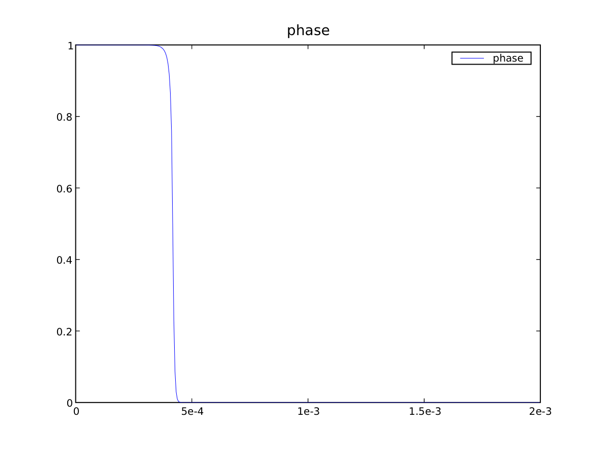
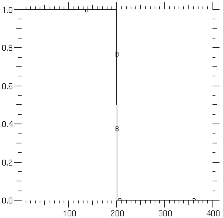
and set a step-function initial condition

$\phi = \begin{cases} 1 & \text{for $x \le L/2$} \\ 0 & \text{for $x > L/2$} \end{cases} \quad\text{at $t = 0$}$

>>> x = mesh.cellCenters[0]
>>> phase.setValue(1.)
>>> phase.setValue(0., where=x > L/2)

If we are running interactively, we’ll want a viewer to see the results

>>> from fipy import input
>>> if __name__ == '__main__':
...     viewer = Viewer(vars = (phase,))
...     viewer.plot()
...     input("Initial condition. Press <return> to proceed...")

We choose the parameter values,

>>> kappa = 0.0025
>>> W = 1.
>>> Lv = 1.
>>> Tm = 1.
>>> T = Tm
>>> enthalpy = Lv * (T - Tm) / Tm

We build the equation by assembling the appropriate terms. Since, with $T = T_M$ we are interested in a steady-state solution, we omit the transient term $(1/M_\phi)\frac{\partial \phi}{\partial t}$ .

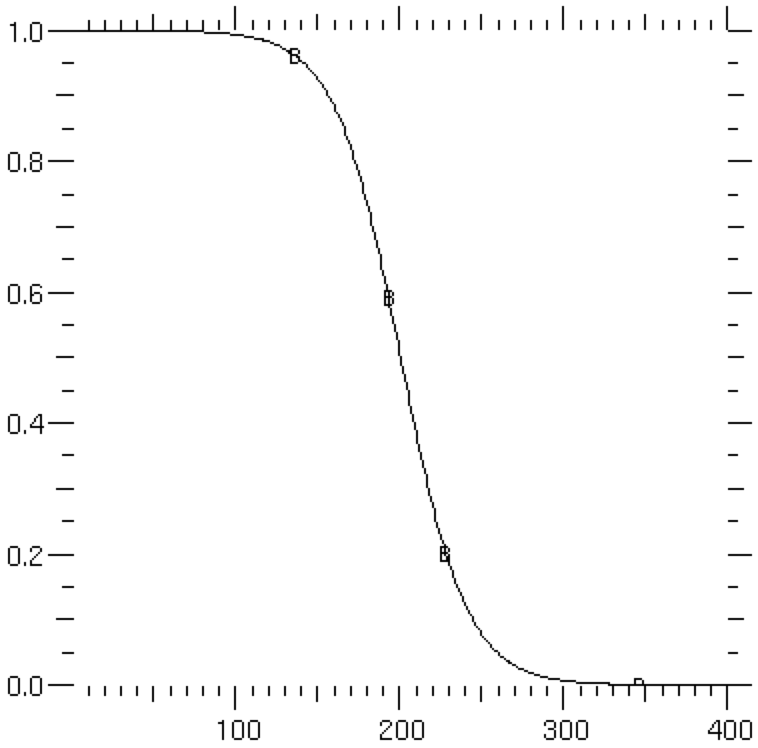
The analytical solution for this steady-state phase field problem, in an infinite domain, is

(2)¶ $\phi = \frac{1}{2}\left[1 - \tanh\frac{x-L/2}{2\sqrt{\kappa/W}}\right]$

or

>>> x = mesh.cellCenters[0]
>>> analyticalArray = 0.5*(1 - numerix.tanh((x - L/2)/(2*numerix.sqrt(kappa/W))))

We treat the diffusion term $\kappa_\phi \nabla^2\phi$ implicitly,

Note

“Diffusion” in FiPy is not limited to the movement of atoms, but rather refers to the spontaneous spreading of any quantity (e.g., solute, temperature, or in this case “phase”) by flow “down” the gradient of that quantity.

The source term is

$S = -\frac{\partial f}{\partial \phi} &= -\frac{W}{2}g'(\phi) - L\frac{T-T_M}{T_M}p'(\phi) \\ &= -\left[W\phi(1-\phi)(1-2\phi) + L\frac{T-T_M}{T_M}30\phi^2(1-\phi)^2\right] \\ &= m_\phi\phi(1-\phi)$

where $m_\phi \equiv -[W(1-2\phi) + 30\phi(1-\phi)L\frac{T-T_M}{T_M}]$ .

The simplest approach is to add this source explicitly

>>> mPhi = -((1 - 2 * phase) * W + 30 * phase * (1 - phase) * enthalpy)
>>> S0 = mPhi * phase * (1 - phase)
>>> eq = S0 + DiffusionTerm(coeff=kappa)

After solving this equation

>>> eq.solve(var = phase, solver=DummySolver())

we obtain the surprising result that $\phi$ is zero everywhere.

>>> print(phase.allclose(analyticalArray, rtol = 1e-4, atol = 1e-4))
0
>>> from fipy import input
>>> if __name__ == '__main__':
...     viewer.plot()
...     input("Fully explicit source. Press <return> to proceed...")

steady-state phase field zero everywhere

On inspection, we can see that this occurs because, for our step-function initial condition, $m_\phi = 0$ everywhere, hence we are actually only solving the simple implicit diffusion equation $\kappa_\phi \nabla^2\phi = 0$ , which has exactly the uninteresting solution we obtained.

The resolution to this problem is to apply relaxation to obtain the desired answer, i.e., the solution is allowed to relax in time from the initial condition to the desired equilibrium solution. To do so, we reintroduce the transient term from Equation (1)

>>> eq = TransientTerm() == DiffusionTerm(coeff=kappa) + S0

>>> phase.setValue(1.)
>>> phase.setValue(0., where=x > L/2)

>>> from builtins import range
>>> for i in range(13):
...     eq.solve(var = phase, dt=1.)
...     if __name__ == '__main__':
...         viewer.plot()

After 13 time steps, the solution has converged to the analytical solution

>>> print(phase.allclose(analyticalArray, rtol = 1e-4, atol = 1e-4))
1
>>> from fipy import input
>>> if __name__ == '__main__':
...     input("Relaxation, explicit. Press <return> to proceed...")

steady-state equilibrium phase field after relaxation

Note

The solution is only found accurate to $\approx 4.3\times 10^{-5}$ because the infinite-domain analytical solution (2) is not an exact representation for the solution in a finite domain of length $L$ .

Setting fixed-value boundary conditions of 1 and 0 would still require the relaxation method with the fully explicit source.

Solution performance can be improved if we exploit the dependence of the source on $\phi$ . By doing so, we can make the source semi-implicit, improving the rate of convergence over the fully explicit approach. The source can only be semi-implicit because we employ sparse linear algebra routines to solve the PDEs, i.e., there is no fully implicit way to represent a term like $\phi^4$ in the linear set of equations $\mathsf{M} \vec{\phi} - \vec{b} = 0$ .

By linearizing a source as $S = S_0 - S_1 \phi$ , we make it more implicit by adding the coefficient $S_1$ to the matrix diagonal. For numerical stability, this linear coefficient must never be negative.

There are an infinite number of choices for this linearization, but many do not converge very well. One choice is that used by Ryo Kobayashi:

>>> S0 = mPhi * phase * (mPhi > 0)
>>> S1 = mPhi * ((mPhi < 0) - phase)
>>> eq = DiffusionTerm(coeff=kappa) + S0 \
...   + ImplicitSourceTerm(coeff = S1)

Note

Because mPhi is a variable field, the quantities (mPhi > 0) and (mPhi < 0) evaluate to variable fields of True and False, instead of single Boolean values.

This expression converges to the same value given by the explicit relaxation approach, but in only 8 sweeps (note that because there is no transient term, these sweeps are not time steps, but rather repeated iterations at the same time step to reach a converged solution).

Note

We use solve() instead of sweep() because we don’t care about the residual. Either function would work, but solve() is a bit faster.

>>> phase.setValue(1.)
>>> phase.setValue(0., where=x > L/2)

>>> from builtins import range
>>> for i in range(8):
...     eq.solve(var = phase)
>>> print(phase.allclose(analyticalArray, rtol = 1e-4, atol = 1e-4))
1
>>> from fipy import input
>>> if __name__ == '__main__':
...     viewer.plot()
...     input("Kobayashi, semi-implicit. Press <return> to proceed...")

In general, the best convergence is obtained when the linearization gives a good representation of the relationship between the source and the dependent variable. The best practical advice is to perform a Taylor expansion of the source about the previous value of the dependent variable such that $S = S_\text{old} + \left.\frac{\partial S}{\partial \phi}\right\rvert_\text{old} (\phi - \phi_\text{old}) = (S - \frac{\partial S}{\partial\phi} \phi)_\text{old} + \left.\frac{\partial S}{\partial \phi}\right|_\text{old} \phi$ . Now, if our source term is represented by $S = S_0 + S_1 \phi$ , then $S_1 = \left.\frac{\partial S}{\partial \phi}\right|_\text{old}$ and $S_0 = (S - \frac{\partial S}{\partial\phi} \phi)_\text{old} = S_\text{old} - S_1 \phi_\text{old}$ . In this way, the linearized source will be tangent to the curve of the actual source as a function of the dependent variable.

For our source, $S = m_\phi \phi (1 - \phi)$ ,

$\frac{\partial S}{\partial \phi} = \frac{\partial m_\phi}{\partial \phi} \phi (1 - \phi) + m_\phi (1 - 2\phi)$

and

$\frac{\partial m_\phi}{\partial \phi} = 2 W - 30 (1 - 2\phi) L\frac{T-T_M}{T_M},$

or

>>> dmPhidPhi = 2 * W - 30 * (1 - 2 * phase) * enthalpy
>>> S1 = dmPhidPhi * phase * (1 - phase) + mPhi * (1 - 2 * phase)
>>> S0 = mPhi * phase * (1 - phase) - S1 * phase
>>> eq = DiffusionTerm(coeff=kappa) + S0 \
...   + ImplicitSourceTerm(coeff = S1)

Using this scheme, where the coefficient of the implicit source term is tangent to the source, we reach convergence in only 5 sweeps

>>> phase.setValue(1.)
>>> phase.setValue(0., where=x > L/2)

>>> from builtins import range
>>> for i in range(5):
...     eq.solve(var = phase)
>>> print(phase.allclose(analyticalArray, rtol = 1e-4, atol = 1e-4))
1
>>> from fipy import input
>>> if __name__ == '__main__':
...     viewer.plot()
...     input("Tangent, semi-implicit. Press <return> to proceed...")

Although, for this simple problem, there is no appreciable difference in run-time between the fully explicit source and the optimized semi-implicit source, the benefit of 60% fewer sweeps should be obvious for larger systems and longer iterations.

This example has focused on just the region of the phase field interface in equilibrium. Problems of interest, though, usually involve the dynamics of one phase transforming to another. To that end, let us recast the problem using physical parameters and dimensions. We’ll need a new mesh

>>> nx = 400
>>> dx = 5e-6 # cm
>>> L = nx * dx

>>> mesh = Grid1D(dx = dx, nx = nx)

and thus must redeclare $\phi$ on the new mesh

>>> phase = CellVariable(name="phase",
...                      mesh=mesh,
...                      hasOld=1)
>>> x = mesh.cellCenters[0]
>>> phase.setValue(1.)
>>> phase.setValue(0., where=x > L/2)

We choose the parameter values appropriate for nickel, given in [23]

>>> Lv = 2350 # J / cm**3
>>> Tm = 1728. # K
>>> T = Variable(value=Tm)
>>> enthalpy = Lv * (T - Tm) / Tm # J / cm**3

The parameters of the phase field model can be related to the surface energy $\sigma$ and the interfacial thickness $\delta$ by

$\kappa &= 6\sigma\delta \\ W &= \frac{6\sigma}{\delta} \\ M_\phi &= \frac{T_m\beta}{6 L \delta}.$

We take $\delta \approx \Delta x$ .

>>> delta = 1.5 * dx
>>> sigma = 3.7e-5 # J / cm**2
>>> beta = 0.33 # cm / (K s)
>>> kappa = 6 * sigma * delta # J / cm
>>> W = 6 * sigma / delta # J / cm**3
>>> Mphi = Tm * beta / (6. * Lv * delta) # cm**3 / (J s)

>>> if __name__ == '__main__':
...     displacement = L * 0.1
... else:
...     displacement = L * 0.025

>>> analyticalArray = CellVariable(name="tanh", mesh=mesh,
...                                value=0.5 * (1 - numerix.tanh((x - (L / 2. + displacement))
...                                                              / (2 * delta))))

and make a new viewer

>>> if __name__ == '__main__':
...     viewer2 = Viewer(vars = (phase, analyticalArray))
...     viewer2.plot()

Now we can redefine the transient phase field equation, using the optimal form of the source term shown above

>>> mPhi = -((1 - 2 * phase) * W + 30 * phase * (1 - phase) * enthalpy)
>>> dmPhidPhi = 2 * W - 30 * (1 - 2 * phase) * enthalpy
>>> S1 = dmPhidPhi * phase * (1 - phase) + mPhi * (1 - 2 * phase)
>>> S0 = mPhi * phase * (1 - phase) - S1 * phase
>>> eq = TransientTerm(coeff=1/Mphi) == DiffusionTerm(coeff=kappa) \
...                         + S0 + ImplicitSourceTerm(coeff = S1)

In order to separate the effect of forming the phase field interface from the kinetics of moving it, we first equilibrate at the melting point. We now use the sweep() method instead of solve() because we require the residual.

>>> timeStep = 1e-6
>>> from builtins import range
>>> for i in range(10):
...     phase.updateOld()
...     res = 1e+10
...     while res > 1e-5:
...         res = eq.sweep(var=phase, dt=timeStep)
>>> if __name__ == '__main__':
...     viewer2.plot()

and then quench by 1 K

>>> T.setValue(T() - 1)

In order to have a stable numerical solution, the interface must not move more than one grid point per time step, we thus set the timestep according to the grid spacing $\Delta x$ , the linear kinetic coefficient $\beta$ , and the undercooling $\abs{T_m - T}$ Again we use the sweep() method as a replacement for solve().

>>> velocity = beta * abs(Tm - T()) # cm / s
>>> timeStep = .1 * dx / velocity # s
>>> elapsed = 0
>>> while elapsed < displacement / velocity:
...     phase.updateOld()
...     res = 1e+10
...     while res > 1e-5:
...         res = eq.sweep(var=phase, dt=timeStep)
...     elapsed += timeStep
...     if __name__ == '__main__':
...         viewer2.plot()

A hyperbolic tangent is not an exact steady-state solution given the quintic polynomial we chose for the $p$ function, but it gives a reasonable approximation.

>>> print(phase.allclose(analyticalArray, rtol = 5, atol = 2e-3))
1

If we had made another common choice of $p(\phi) = \phi^2(3 - 2\phi)$ , we would have found much better agreement, as that case does give an exact $\tanh$ solution in steady state. If SciPy is available, another way to compare against the expected result is to do a least-squared fit to determine the interface velocity and thickness

>>> try:
...     def tanhResiduals(p, y, x, t):
...         V, d = p
...         return y - 0.5 * (1 - numerix.tanh((x - V * t - L / 2.) / (2*d)))
...     from scipy.optimize import leastsq 
...     x =  mesh.cellCenters[0]
...     (V_fit, d_fit), msg = leastsq(tanhResiduals, [L/2., delta],
...                                   args=(phase.globalValue, x.globalValue, elapsed)) 
... except ImportError:
...     V_fit = d_fit = 0
...     print("The SciPy library is unavailable to fit the interface \
... thickness and velocity")

>>> print(abs(1 - V_fit / velocity) < 4.1e-2) 
True
>>> print(abs(1 - d_fit / delta) < 2e-2) 
True

>>> from fipy import input
>>> if __name__ == '__main__':
...     input("Dimensional, semi-implicit. Press <return> to proceed...")

phase field when solved with physical parameters

Last updated on Jun 27, 2023. Created using Sphinx 6.2.1.