 FiPy
FiPyFinite Volume Method
To use the FVM, the solution domain must first be divided into
non-overlapping polyhedral elements or cells. A solution domain
divided in such a way is generally known as a mesh (as we will see, a
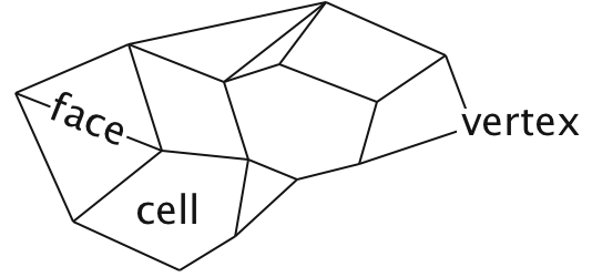
Mesh is also a FiPy object). A mesh consists of vertices,
faces and cells (see Figure Mesh). In the FVM the
variables of interest are averaged over control volumes (CVs). The
CVs are either defined by the cells or are centered on the vertices.
Mesh
A mesh consists of cells, faces and vertices. For the purposes of FiPy, the divider between two cells is known as a face for all dimensions.
Cell Centered FVM (CC-FVM)
In the CC-FVM the CVs are formed by the mesh cells with the cell center “storing” the average variable value in the CV, (see Figure CV structure for an unstructured mesh). The face fluxes are approximated using the variable values in the two adjacent cells surrounding the face. This low order approximation has the advantage of being efficient and requiring matrices of low band width (the band width is equal to the number of cell neighbors plus one) and thus low storage requirement. However, the mesh topology is restricted due to orthogonality and conjunctionality requirements. The value at a face is assumed to be the average value over the face. On an unstructured mesh the face center may not lie on the line joining the CV centers, which will lead to an error in the face interpolation. FiPy currently only uses the CC-FVM.
Boundary Conditions
The natural boundary condition for CC-FVM is no-flux. For (2), the boundary condition is
![\hat{n}\cdot[\vec{u}\phi - (\Gamma_i\nabla)^n] = 0](../../_images/math/bcdc5acd317058911eaff347fd4234ee8592c259.svg)
Vertex Centered FVM (VC-FVM)
In the VC-FVM, the CV is centered around the vertices and the cells are divided into sub-control volumes that make up the main CVs (see Figure CV structure for an unstructured mesh). The vertices “store” the average variable values over the CVs. The CV faces are constructed within the cells rather than using the cell faces as in the CC-FVM. The face fluxes use all the vertex values from the cell where the face is located to calculate interpolations. For this reason, the VC-FVM is less efficient and requires more storage (a larger matrix band width) than the CC-FVM. However, the mesh topology does not have the same restrictions as the CC-FVM. FiPy does not have a VC-FVM capability.

CV structure for an unstructured mesh
(a)  represents a vertex-based CV and (b)
 ,
,  ,
,  and
and
 represent cell centered CVs.
Discretization
The first step in the discretization of Equation (2) using the CC-FVM is to integrate over a CV and then make appropriate approximations for fluxes across the boundary of each CV. In this section, each term in Equation (2) will be examined separately.
Transient Term  
For the transient term, the discretization of the integral  over the volume of a CV is given by
(1)
where  represents the average value of
  in a CV
centered on a point
in a CV
centered on a point  and the superscript “
 ”
represents the previous time-step value. The value
”
represents the previous time-step value. The value  is the
volume of the CV and
is the
volume of the CV and  is the time step size.
This term is represented in FiPy as
>>> TransientTerm(coeff=rho)
Convection Term  
The discretization for the convection term is given by
(2)
where we have used the divergence theorem to transform the integral
over the CV volume into an integral over the CV surface
 . The summation over the faces of a CV is denoted by
 and
and  is the area of each face. The vector
  is the normal to the face pointing out of the CV into an adjacent CV
centered on point
is the normal to the face pointing out of the CV into an adjacent CV
centered on point  . When using a first order approximation,
the value of
. When using a first order approximation,
the value of  must depend on the average value in adjacent
cell
must depend on the average value in adjacent
cell  and the average value in the cell of interest ,
such that
and the average value in the cell of interest ,
such that

The weighting factor  is determined by the convection
scheme, described in Numerical Schemes.
is determined by the convection
scheme, described in Numerical Schemes.
This term is represented in FiPy as
>>> <SpecificConvectionTerm>(coeff=u)
where <SpecificConvectionTerm> can be any of
CentralDifferenceConvectionTerm,
ExponentialConvectionTerm,
HybridConvectionTerm,
PowerLawConvectionTerm,
UpwindConvectionTerm,
ExplicitUpwindConvectionTerm, or
VanLeerConvectionTerm.
The differences between these convection schemes are described
in Section Numerical Schemes. The velocity coefficient
u must be a rank-1 FaceVariable, or a
constant vector in the form of a Python list or
tuple, e.g. ((1,), (2,)) for a vector in 2D.
Diffusion Term  
The discretization for the diffusion term is given by
(3)
 indicates recursive application of the specified
operation on , depending on
the order of the diffusion term.
The estimation for the flux,
indicates recursive application of the specified
operation on , depending on
the order of the diffusion term.
The estimation for the flux,  , is
obtained via
, is
obtained via

where the value of  is the distance between neighboring cell
centers. This estimate relies on the orthogonality of the mesh, and
becomes increasingly inaccurate as the non-orthogonality increases.
Correction terms have been derived to improve this error but are not
currently included in FiPy [14].
is the distance between neighboring cell
centers. This estimate relies on the orthogonality of the mesh, and
becomes increasingly inaccurate as the non-orthogonality increases.
Correction terms have been derived to improve this error but are not
currently included in FiPy [14].
This term is represented in FiPy as
>>> DiffusionTerm(coeff=Gamma1)
or
>>> ExplicitDiffusionTerm(coeff=Gamma1)
ExplicitDiffusionTerm is provided primarily for
illustrative purposes, although examples.diffusion.mesh1D
demonstrates its use in Crank-Nicolson time stepping.
ImplicitDiffusionTerm is almost always
preferred (DiffusionTerm is a synonym for
ImplicitDiffusionTerm to reinforce this
preference). One can also create an explicit diffusion term with
>>> (Gamma1 * phi.faceGrad).divergence
Higher Order Diffusion
Higher order diffusion expressions, such as  or
or
 for Cahn-Hilliard are
represented as
for Cahn-Hilliard are
represented as
>>> DiffusionTerm(coeff=(Gamma1, Gamma2))
The number of elements supplied for coeff determines the
order of the term.
Note
While this multiple-coefficient form is still supported, Coupled and Vector Equations are the recommended approach for higher order expressions.
Source Term
Any term that cannot be written in one of the previous forms is considered
a source  . The discretization for the source term is given
by,
. The discretization for the source term is given
by,
(4)
Including any negative dependence of  on increases
solution stability. The dependence can only be included in a linear
manner so Equation (4) becomes
on increases
solution stability. The dependence can only be included in a linear
manner so Equation (4) becomes

where  is the source which is independent of and
 is the coefficient of the source which is linearly dependent
on .
is the coefficient of the source which is linearly dependent
on .
A source term is represented in FiPy essentially as it appears in
mathematical form, e.g.,  would be written
>>> 3 * kappa**2 + b * numerix.sin(theta)
Note
Functions like sin() can be obtained from the
fipy.tools.numerix module.
If, however, the source depends on the variable that is being solved for,
it can be advantageous to linearize the source and cast part of it as an
implicit source term, e.g.,  might be written as
>>> 3 * kappa**2 + ImplicitSourceTerm(coeff=sin(theta))
Linear Equations
The aim of the discretization is to reduce the continuous general equation to a set of discrete linear equations that can then be solved to obtain the value of the dependent variable at each CV center. This results in a sparse linear system that requires an efficient iterative scheme to solve. The iterative schemes available to FiPy are currently encapsulated in the Pysparse and PyTrilinos suites of solvers and include most common solvers such as the conjugate gradient method and LU decomposition.
Combining Equations (1), (2), (3) and (4), the complete discretization for equation (2) can now be written for each CV as
(5)¶![\frac{\rho_{P}(\phi_{P} - \phi_P^\text{old}) V_P}{\Delta t}
+ &
\sum_{f} (\vec{n} \cdot \vec{u})_f A_f
\left[\alpha_f \phi_P +\left(1-\alpha_f\right)\phi_A\right]
\nonumber \\
= &
\sum_f \Gamma_f A_f \frac{(\phi_A-\phi_P)}{d_{AP}}
+
V_P ( S_0 + S_1 \phi_P ).](../../_images/math/1eeb6c1f05a4a180896c528c8b2c79e3681a64d1.svg)
Equation (5) is now in the form of a set of linear combinations between each CV value and its neighboring values and can be written in the form
(6)
where

The face coefficients,  and
and  , represent the convective strength
and diffusive conductance respectively, and are given by
, represent the convective strength
and diffusive conductance respectively, and are given by
