variables Package¶

`variables` Package¶

class fipy.variables.Variable(value=0.0, unit=None, array=None, name='', cached=1)¶

Bases: object

Lazily evaluated quantity with units.

Using a Variable in a mathematical expression will create an automatic dependency Variable, e.g.,

>>> a = Variable(value=3)
>>> b = 4 * a
>>> b
(Variable(value=array(3)) * 4)
>>> b()
12

Changes to the value of a Variable will automatically trigger changes in any dependent Variable objects

>>> a.setValue(5)
>>> b
(Variable(value=array(5)) * 4)
>>> print b()
20

Create a Variable.

>>> Variable(value=3)
Variable(value=array(3))
>>> Variable(value=3, unit="m")
Variable(value=PhysicalField(3,'m'))
>>> Variable(value=3, unit="m", array=numerix.zeros((3,2), 'l'))
Variable(value=PhysicalField(array([[3, 3],
       [3, 3],
       [3, 3]]),'m'))

Parameters :	value: the initial value unit: the physical units of the Variable array: the storage array for the Variable name: the user-readable name of the Variable cached: whether to cache or always recalculate the value

all(axis=None)¶

>>> print Variable(value=(0, 0, 1, 1)).all()
0
>>> print Variable(value=(1, 1, 1, 1)).all()
1

allclose(other, rtol=1e-05, atol=1e-08)¶

>>> var = Variable((1, 1))
   >>> print var.allclose((1, 1))
   1
   >>> print var.allclose((1,))
   1

The following test is to check that the system does not run out of memory.

>>> from fipy.tools import numerix
>>> var = Variable(numerix.ones(10000))
>>> print var.allclose(numerix.zeros(10000, 'l'))
False

allequal(other)¶

any(axis=None)¶

>>> print Variable(value=0).any()
0
>>> print Variable(value=(0, 0, 1, 1)).any()
1

arccos(*args, **kwds)¶: Deprecated since version 3.0: use numerix.arccos() instead

arccosh(*args, **kwds)¶: Deprecated since version 3.0: use numerix.arccosh() instead

arcsin(*args, **kwds)¶: Deprecated since version 3.0: use numerix.arcsin() instead

arcsinh(*args, **kwds)¶: Deprecated since version 3.0: use numerix.arcsinh() instead

arctan(*args, **kwds)¶: Deprecated since version 3.0: use numerix.arctan() instead

arctan2(*args, **kwds)¶: Deprecated since version 3.0: use numerix.arctan2() instead

arctanh(*args, **kwds)¶: Deprecated since version 3.0: use numerix.arctanh() instead

cacheMe(recursive=False)¶

ceil(*args, **kwds)¶: Deprecated since version 3.0: use numerix.ceil() instead

conjugate(*args, **kwds)¶: Deprecated since version 3.0: use numerix.conjugate() instead

constrain(value, where=None)¶

Constrain the Variable to have a value at an index or mask location specified by where.

>>> v = Variable((0,1,2,3))
>>> v.constrain(2, numerix.array((True, False, False, False)))
>>> print v
[2 1 2 3]
>>> v[:] = 10
>>> print v
[ 2 10 10 10]
>>> v.constrain(5, numerix.array((False, False, True, False)))
>>> print v
[ 2 10  5 10]
>>> v[:] = 6
>>> print v
[2 6 5 6]
>>> v.constrain(8)
>>> print v
[8 8 8 8]
>>> v[:] = 10
>>> print v
[8 8 8 8]
>>> del v.constraints[2]
>>> print v
[ 2 10  5 10]

>>> from fipy.variables.cellVariable import CellVariable
>>> from fipy.meshes import Grid2D
>>> m = Grid2D(nx=2, ny=2)
>>> x, y = m.cellCenters
>>> v = CellVariable(mesh=m, rank=1, value=(x, y))
>>> v.constrain(((0.,), (-1.,)), where=m.facesLeft)
>>> print v.faceValue
[[ 0.5  1.5  0.5  1.5  0.5  1.5  0.   1.   1.5  0.   1.   1.5]
 [ 0.5  0.5  1.   1.   1.5  1.5 -1.   0.5  0.5 -1.   1.5  1.5]]

Parameters :	value: the value of the constraint where: the constraint mask or index specifying the location of the constraint

constraints¶

copy()¶

Make an duplicate of the Variable

>>> a = Variable(value=3)
>>> b = a.copy()
>>> b
Variable(value=array(3))

The duplicate will not reflect changes made to the original

>>> a.setValue(5)
>>> b
Variable(value=array(3))

Check that this works for arrays.

>>> a = Variable(value=numerix.array((0,1,2)))
>>> b = a.copy()
>>> b
Variable(value=array([0, 1, 2]))
>>> a[1] = 3
>>> b
Variable(value=array([0, 1, 2]))

cos(*args, **kwds)¶: Deprecated since version 3.0: use numerix.cos() instead

cosh(*args, **kwds)¶: Deprecated since version 3.0: use numerix.cosh() instead

dontCacheMe(recursive=False)¶

dot(other, opShape=None, operatorClass=None, axis=0)¶

exp(*args, **kwds)¶: Deprecated since version 3.0: use numerix.exp() instead

floor(*args, **kwds)¶: Deprecated since version 3.0: use numerix.floor() instead

getMag(*args, **kwds)¶: Deprecated since version 3.0: use the mag property instead

getName(*args, **kwds)¶: Deprecated since version 3.0: use the name property instead

getNumericValue(*args, **kwds)¶: Deprecated since version 3.0: use the numericValue property instead

getShape(*args, **kwds)¶: Deprecated since version 3.0: use the shape property instead

getSubscribedVariables(*args, **kwds)¶: Deprecated since version 3.0: use the subscribedVariables property instead

getUnit(*args, **kwds)¶: Deprecated since version 3.0: use the unit property instead

getValue(*args, **kwds)¶: Deprecated since version 3.0: use the value property instead

getsctype(default=None)¶

Returns the Numpy sctype of the underlying array.

>>> Variable(1).getsctype() == numerix.NUMERIX.obj2sctype(numerix.array(1))
True
>>> Variable(1.).getsctype() == numerix.NUMERIX.obj2sctype(numerix.array(1.))
True
>>> Variable((1,1.)).getsctype() == numerix.NUMERIX.obj2sctype(numerix.array((1., 1.)))
True

inBaseUnits()¶

Return the value of the Variable with all units reduced to their base SI elements.

>>> e = Variable(value="2.7 Hartree*Nav")
>>> print e.inBaseUnits().allclose("7088849.01085 kg*m**2/s**2/mol")
1

inUnitsOf(*units)¶

Returns one or more Variable objects that express the same physical quantity in different units. The units are specified by strings containing their names. The units must be compatible with the unit of the object. If one unit is specified, the return value is a single Variable.

>>> freeze = Variable('0 degC')
>>> print freeze.inUnitsOf('degF').allclose("32.0 degF")
1

If several units are specified, the return value is a tuple of Variable instances with with one element per unit such that the sum of all quantities in the tuple equals the the original quantity and all the values except for the last one are integers. This is used to convert to irregular unit systems like hour/minute/second. The original object will not be changed.

>>> t = Variable(value=314159., unit='s')
>>> print numerix.allclose([e.allclose(v) for (e, v) in zip(t.inUnitsOf('d','h','min','s'),
...                                                         ['3.0 d', '15.0 h', '15.0 min', '59.0 s'])], 
...                        True)
1

itemset(value)¶

itemsize¶

log(*args, **kwds)¶: Deprecated since version 3.0: use numerix.log() instead

log10(*args, **kwds)¶: Deprecated since version 3.0: use numerix.log10() instead

mag¶

max(axis=None)¶

min(axis=None)¶

name¶

numericValue¶

put(indices, value)¶

ravel()¶

release(constraint)¶

Remove constraint from self

>>> v = Variable((0,1,2,3))
>>> v.constrain(2, numerix.array((True, False, False, False)))
>>> v[:] = 10
>>> from fipy.boundaryConditions.constraint import Constraint
>>> c1 = Constraint(5, numerix.array((False, False, True, False)))
>>> v.constrain(c1)
>>> v[:] = 6
>>> v.constrain(8)
>>> v[:] = 10
>>> del v.constraints[2]
>>> v.release(constraint=c1)
>>> print v
[ 2 10 10 10]

reshape(*args, **kwds)¶: Deprecated since version 3.0: use numerix.reshape() instead

setName(*args, **kwds)¶: Deprecated since version 3.0: use the name property instead

setUnit(*args, **kwds)¶: Deprecated since version 3.0: use the unit property instead

setValue(value, unit=None, where=None)¶

Set the value of the Variable. Can take a masked array.

>>> a = Variable((1,2,3))
>>> a.setValue(5, where=(1, 0, 1))
>>> print a
[5 2 5]

>>> b = Variable((4,5,6))
>>> a.setValue(b, where=(1, 0, 1))
>>> print a
[4 2 6]
>>> print b
[4 5 6]
>>> a.value = 3
>>> print a
[3 3 3]

>>> b = numerix.array((3,4,5))
>>> a.value = b
>>> a[:] = 1
>>> print b
[3 4 5]

>>> a.setValue((4,5,6), where=(1, 0)) 
Traceback (most recent call last):
    ....
ValueError: shape mismatch: objects cannot be broadcast to a single shape

shape¶

Tuple of array dimensions.

>>> Variable(value=3).shape
()
>>> Variable(value=(3,)).shape
(1,)
>>> Variable(value=(3,4)).shape
(2,)

>>> Variable(value="3 m").shape
()
>>> Variable(value=(3,), unit="m").shape
(1,)
>>> Variable(value=(3,4), unit="m").shape
(2,)

sign(*args, **kwds)¶: Deprecated since version 3.0: use numerix.sign() instead

sin(*args, **kwds)¶: Deprecated since version 3.0: use numerix.sin() instead

sinh(*args, **kwds)¶: Deprecated since version 3.0: use numerix.sinh() instead

sqrt(*args, **kwds)¶

Deprecated since version 3.0: use numerix.sqrt() instead

>>> from fipy.meshes import Grid1D
>>> mesh= Grid1D(nx=3)

>>> from fipy.variables.cellVariable import CellVariable
>>> var = CellVariable(mesh=mesh, value=((0., 2., 3.),), rank=1)
>>> print (var.dot(var)).sqrt()
[ 0.  2.  3.]

subscribedVariables¶

sum(axis=None)¶

take(ids, axis=0)¶

tan(*args, **kwds)¶: Deprecated since version 3.0: use numerix.tan() instead

tanh(*args, **kwds)¶: Deprecated since version 3.0: use numerix.tanh() instead

tostring(max_line_width=75, precision=8, suppress_small=False, separator=' ')¶

unit¶

Return the unit object of self.

>>> Variable(value="1 m").unit
<PhysicalUnit m>

value¶

“Evaluate” the Variable and return its value (longhand)

>>> a = Variable(value=3)
>>> print a.value
3
>>> b = a + 4
>>> b
(Variable(value=array(3)) + 4)
>>> b.value
7

class fipy.variables.CellVariable(mesh, name='', value=0.0, rank=None, elementshape=None, unit=None, hasOld=0)¶

Bases: fipy.variables.meshVariable._MeshVariable

Represents the field of values of a variable on a Mesh.

A CellVariable can be pickled to persistent storage (disk) for later use:

>>> from fipy.meshes import Grid2D
>>> mesh = Grid2D(dx = 1., dy = 1., nx = 10, ny = 10)

>>> var = CellVariable(mesh = mesh, value = 1., hasOld = 1, name = 'test')
>>> x, y = mesh.cellCenters
>>> var.value = (x * y)

>>> from fipy.tools import dump        
>>> (f, filename) = dump.write(var, extension = '.gz')
>>> unPickledVar = dump.read(filename, f)

>>> print var.allclose(unPickledVar, atol = 1e-10, rtol = 1e-10)
1

arithmeticFaceValue¶

Returns a FaceVariable whose value corresponds to the arithmetic interpolation of the adjacent cells:

$\phi_f = (\phi_1 - \phi_2) \frac{d_{f2}}{d_{12}} + \phi_2$

>>> from fipy.meshes import Grid1D
>>> from fipy import numerix
>>> mesh = Grid1D(dx = (1., 1.))
>>> L = 1
>>> R = 2
>>> var = CellVariable(mesh = mesh, value = (L, R))
>>> faceValue = var.arithmeticFaceValue[mesh.interiorFaces.value]
>>> answer = (R - L) * (0.5 / 1.) + L
>>> print numerix.allclose(faceValue, answer, atol = 1e-10, rtol = 1e-10)
True

>>> mesh = Grid1D(dx = (2., 4.))
>>> var = CellVariable(mesh = mesh, value = (L, R))
>>> faceValue = var.arithmeticFaceValue[mesh.interiorFaces.value]
>>> answer = (R - L) * (1.0 / 3.0) + L
>>> print numerix.allclose(faceValue, answer, atol = 1e-10, rtol = 1e-10)
True

>>> mesh = Grid1D(dx = (10., 100.))
>>> var = CellVariable(mesh = mesh, value = (L, R))
>>> faceValue = var.arithmeticFaceValue[mesh.interiorFaces.value]
>>> answer = (R - L) * (5.0 / 55.0) + L
>>> print numerix.allclose(faceValue, answer, atol = 1e-10, rtol = 1e-10)
True

cellVolumeAverage¶

Return the cell-volume-weighted average of the CellVariable:

$<\phi>_\text{vol} = \frac{\sum_\text{cells} \phi_\text{cell} V_\text{cell}} {\sum_\text{cells} V_\text{cell}}$

>>> from fipy.meshes import Grid2D
>>> from fipy.variables.cellVariable import CellVariable
>>> mesh = Grid2D(nx = 3, ny = 1, dx = .5, dy = .1)
>>> var = CellVariable(value = (1, 2, 6), mesh = mesh)
>>> print var.cellVolumeAverage
3.0

constrain(value, where=None)¶

Constrains the CellVariable to value at a location specified by where.

>>> from fipy import *
>>> m = Grid1D(nx=3)
>>> v = CellVariable(mesh=m, value=m.cellCenters[0])
>>> v.constrain(0., where=m.facesLeft)
>>> v.faceGrad.constrain([1.], where=m.facesRight)
>>> print v.faceGrad
[[ 1.  1.  1.  1.]]
>>> print v.faceValue
[ 0.   1.   2.   2.5]

Changing the constraint changes the dependencies

>>> v.constrain(1., where=m.facesLeft)
>>> print v.faceGrad
[[-1.  1.  1.  1.]]
>>> print v.faceValue
[ 1.   1.   2.   2.5]

Constraints can be Variable

>>> c = Variable(0.)
>>> v.constrain(c, where=m.facesLeft)
>>> print v.faceGrad
[[ 1.  1.  1.  1.]]
>>> print v.faceValue
[ 0.   1.   2.   2.5]
>>> c.value = 1.
>>> print v.faceGrad
[[-1.  1.  1.  1.]]
>>> print v.faceValue
[ 1.   1.   2.   2.5]

Constraints can have a Variable mask.

>>> v = CellVariable(mesh=m)
>>> mask = FaceVariable(mesh=m, value=m.facesLeft)
>>> v.constrain(1., where=mask)
>>> print v.faceValue
[ 1.  0.  0.  0.]
>>> mask[:] = mask | m.facesRight
>>> print v.faceValue
[ 1.  0.  0.  1.]

copy()¶

faceGrad¶: Return $\nabla \phi$ as a rank-1 FaceVariable using differencing for the normal direction(second-order gradient).

faceGradAverage¶: Return $\nabla \phi$ as a rank-1 FaceVariable using averaging for the normal direction(second-order gradient)

faceValue¶

Returns a FaceVariable whose value corresponds to the arithmetic interpolation of the adjacent cells:

$\phi_f = (\phi_1 - \phi_2) \frac{d_{f2}}{d_{12}} + \phi_2$

>>> from fipy.meshes import Grid1D
>>> from fipy import numerix
>>> mesh = Grid1D(dx = (1., 1.))
>>> L = 1
>>> R = 2
>>> var = CellVariable(mesh = mesh, value = (L, R))
>>> faceValue = var.arithmeticFaceValue[mesh.interiorFaces.value]
>>> answer = (R - L) * (0.5 / 1.) + L
>>> print numerix.allclose(faceValue, answer, atol = 1e-10, rtol = 1e-10)
True

>>> mesh = Grid1D(dx = (2., 4.))
>>> var = CellVariable(mesh = mesh, value = (L, R))
>>> faceValue = var.arithmeticFaceValue[mesh.interiorFaces.value]
>>> answer = (R - L) * (1.0 / 3.0) + L
>>> print numerix.allclose(faceValue, answer, atol = 1e-10, rtol = 1e-10)
True

>>> mesh = Grid1D(dx = (10., 100.))
>>> var = CellVariable(mesh = mesh, value = (L, R))
>>> faceValue = var.arithmeticFaceValue[mesh.interiorFaces.value]
>>> answer = (R - L) * (5.0 / 55.0) + L
>>> print numerix.allclose(faceValue, answer, atol = 1e-10, rtol = 1e-10)
True

gaussGrad¶: Return $\frac{1}{V_P} \sum_f \vec{n} \phi_f A_f$ as a rank-1 CellVariable (first-order gradient).

getArithmeticFaceValue(*args, **kwds)¶: Deprecated since version 3.0: use the arithmeticFaceValue property instead

getCellVolumeAverage(*args, **kwds)¶: Deprecated since version 3.0: use the cellVolumeAverage property instead

getFaceGrad(*args, **kwds)¶: Deprecated since version 3.0: use the faceGrad property instead

getFaceGradAverage(*args, **kwds)¶: Deprecated since version 3.0: use the faceGradAverage property instead

getFaceValue(*args, **kwds)¶: Deprecated since version 3.0: use the arithmeticFaceValue property instead

getGaussGrad(*args, **kwds)¶: Deprecated since version 3.0: use the gaussGrad property instead

getGrad(*args, **kwds)¶: Deprecated since version 3.0: use the grad property instead

getHarmonicFaceValue(*args, **kwds)¶: Deprecated since version 3.0: use the harmonicFaceValue property instead

getLeastSquaresGrad(*args, **kwds)¶: Deprecated since version 3.0: use the leastSquaresGrad property instead

getMinmodFaceValue(*args, **kwds)¶: Deprecated since version 3.0: use the minmodFaceValue property instead

getOld(*args, **kwds)¶: Deprecated since version 3.0: use the old property instead

globalValue¶

Concatenate and return values from all processors

When running on a single processor, the result is identical to value.

grad¶: Return $\nabla \phi$ as a rank-1 CellVariable (first-order gradient).

harmonicFaceValue¶

Returns a FaceVariable whose value corresponds to the harmonic interpolation of the adjacent cells:

$\phi_f = \frac{\phi_1 \phi_2}{(\phi_2 - \phi_1) \frac{d_{f2}}{d_{12}} + \phi_1}$

>>> from fipy.meshes import Grid1D
>>> from fipy import numerix
>>> mesh = Grid1D(dx = (1., 1.))
>>> L = 1
>>> R = 2
>>> var = CellVariable(mesh = mesh, value = (L, R))
>>> faceValue = var.harmonicFaceValue[mesh.interiorFaces.value]
>>> answer = L * R / ((R - L) * (0.5 / 1.) + L)
>>> print numerix.allclose(faceValue, answer, atol = 1e-10, rtol = 1e-10)
True

>>> mesh = Grid1D(dx = (2., 4.))
>>> var = CellVariable(mesh = mesh, value = (L, R))
>>> faceValue = var.harmonicFaceValue[mesh.interiorFaces.value]
>>> answer = L * R / ((R - L) * (1.0 / 3.0) + L)
>>> print numerix.allclose(faceValue, answer, atol = 1e-10, rtol = 1e-10)
True

>>> mesh = Grid1D(dx = (10., 100.))
>>> var = CellVariable(mesh = mesh, value = (L, R))
>>> faceValue = var.harmonicFaceValue[mesh.interiorFaces.value]
>>> answer = L * R / ((R - L) * (5.0 / 55.0) + L)
>>> print numerix.allclose(faceValue, answer, atol = 1e-10, rtol = 1e-10)
True

leastSquaresGrad¶

Return $\nabla \phi$ , which is determined by solving for $\nabla \phi$ in the following matrix equation,

$\nabla \phi \cdot \sum_f d_{AP}^2 \vec{n}_{AP} \otimes \vec{n}_{AP} = \sum_f d_{AP}^2 \left( \vec{n} \cdot \nabla \phi \right)_{AP}$

The matrix equation is derived by minimizing the following least squares sum,

$F \left( \phi_x, \phi_y \right) = \sqrt{\sum_f \left( d_{AP} \vec{n}_{AP} \cdot \nabla \phi - d_{AP} \left( \vec{n}_{AP} \cdot \nabla \phi \right)_{AP} \right)^2 }$

Tests

>>> from fipy import Grid2D
>>> m = Grid2D(nx=2, ny=2, dx=0.1, dy=2.0)
>>> print numerix.allclose(CellVariable(mesh=m, value=(0,1,3,6)).leastSquaresGrad.globalValue, \
...                                     [[8.0, 8.0, 24.0, 24.0],
...                                      [1.2, 2.0, 1.2, 2.0]])
True

>>> from fipy import Grid1D
>>> print numerix.allclose(CellVariable(mesh=Grid1D(dx=(2.0, 1.0, 0.5)), 
...                                     value=(0, 1, 2)).leastSquaresGrad.globalValue, [[0.461538461538, 0.8, 1.2]])
True

minmodFaceValue¶

Returns a FaceVariable with a value that is the minimum of the absolute values of the adjacent cells. If the values are of opposite sign then the result is zero:

$\phi_f = \begin{cases} \phi_1& \text{when $|\phi_1| \le |\phi_2|$},\\ \phi_2& \text{when $|\phi_2| < |\phi_1|$},\\ 0 & \text{when $\phi1 \phi2 < 0$} \end{cases}$

>>> from fipy import *
>>> print CellVariable(mesh=Grid1D(nx=2), value=(1, 2)).minmodFaceValue
[1 1 2]
>>> print CellVariable(mesh=Grid1D(nx=2), value=(-1, -2)).minmodFaceValue
[-1 -1 -2]
>>> print CellVariable(mesh=Grid1D(nx=2), value=(-1, 2)).minmodFaceValue
[-1  0  2]

old¶

Return the values of the CellVariable from the previous solution sweep.

Combinations of CellVariable’s should also return old values.

>>> from fipy.meshes import Grid1D
>>> mesh = Grid1D(nx = 2)
>>> from fipy.variables.cellVariable import CellVariable
>>> var1 = CellVariable(mesh = mesh, value = (2, 3), hasOld = 1)
>>> var2 = CellVariable(mesh = mesh, value = (3, 4))
>>> v = var1 * var2
>>> print v
[ 6 12]
>>> var1.value = ((3,2))
>>> print v
[9 8]
>>> print v.old
[ 6 12]

The following small test is to correct for a bug when the operator does not just use variables.

>>> v1 = var1 * 3
>>> print v1
[9 6]
>>> print v1.old
[6 9]

release(constraint)¶

Remove constraint from self

>>> from fipy import *
>>> m = Grid1D(nx=3)
>>> v = CellVariable(mesh=m, value=m.cellCenters[0])
>>> c = Constraint(0., where=m.facesLeft)
>>> v.constrain(c)
>>> print v.faceValue
[ 0.   1.   2.   2.5]
>>> v.release(constraint=c)
>>> print v.faceValue
[ 0.5  1.   2.   2.5]

setValue(value, unit=None, where=None)¶

updateOld()¶

Set the values of the previous solution sweep to the current values.

>>> from fipy import *
>>> v = CellVariable(mesh=Grid1D(), hasOld=False)
>>> v.updateOld()
Traceback (most recent call last):
   ...
AssertionError: The updateOld method requires the CellVariable to have an old value. Set hasOld to True when instantiating the CellVariable.

class fipy.variables.FaceVariable(mesh, name='', value=0.0, rank=None, elementshape=None, unit=None, cached=1)¶

Bases: fipy.variables.meshVariable._MeshVariable

Parameters :	mesh: the mesh that defines the geometry of this Variable name: the user-readable name of the Variable value: the initial value rank: the rank (number of dimensions) of each element of this Variable. Default: 0 elementshape: the shape of each element of this variable Default: rank * (mesh.dim,) unit: the physical units of the Variable

copy()¶

divergence¶

>>> from fipy.meshes import Grid2D
>>> from fipy.variables.cellVariable import CellVariable
>>> mesh = Grid2D(nx=3, ny=2)
>>> var = CellVariable(mesh=mesh, value=range(3*2))
>>> print var.faceGrad.divergence
[ 4.  3.  2. -2. -3. -4.]

getDivergence(*args, **kwds)¶: Deprecated since version 3.0: use the divergence property instead

globalValue¶

setValue(value, unit=None, where=None)¶

class fipy.variables.ScharfetterGummelFaceVariable(var, boundaryConditions=())¶: Bases: fipy.variables.cellToFaceVariable._CellToFaceVariable

class fipy.variables.ModularVariable(mesh, name='', value=0.0, rank=None, elementshape=None, unit=None, hasOld=0)¶

Bases: fipy.variables.cellVariable.CellVariable

The ModularVariable defines a variable that exisits on the circle between $-\pi$ and $\pi$

The following examples show how ModularVariable works. When subtracting the answer wraps back around the circle.

>>> from fipy.meshes import Grid1D
>>> mesh = Grid1D(nx = 2)
>>> from fipy.tools import numerix
>>> pi = numerix.pi
>>> v1 = ModularVariable(mesh = mesh, value = (2*pi/3, -2*pi/3))
>>> v2 = ModularVariable(mesh = mesh, value = -2*pi/3)
>>> print numerix.allclose(v2 - v1, (2*pi/3, 0))
1

Obtaining the arithmetic face value.

>>> print numerix.allclose(v1.arithmeticFaceValue, (2*pi/3, pi, -2*pi/3))
1

Obtaining the gradient.

>>> print numerix.allclose(v1.grad, ((pi/3, pi/3),))
1

Obtaining the gradient at the faces.

>>> print numerix.allclose(v1.faceGrad, ((0, 2*pi/3, 0),))
1

Obtaining the gradient at the faces but without modular arithmetic.

>>> print numerix.allclose(v1.faceGradNoMod, ((0, -4*pi/3, 0),))
1

arithmeticFaceValue¶

Returns a FaceVariable whose value corresponds to the arithmetic interpolation of the adjacent cells:

$\phi_f = (\phi_1 - \phi_2) \frac{d_{f2}}{d_{12}} + \phi_2$

Adjusted for a ModularVariable

faceGrad¶: Return $\nabla \phi$ as a rank-1 FaceVariable (second-order gradient). Adjusted for a ModularVariable

faceGradNoMod¶: Return $\nabla \phi$ as a rank-1 FaceVariable (second-order gradient). Not adjusted for a ModularVariable

getFaceGradNoMod(*args, **kwds)¶: Deprecated since version 3.0: use the faceGradNoMod property instead

grad¶: Return $\nabla \phi$ as a rank-1 CellVariable (first-order gradient). Adjusted for a ModularVariable

updateOld()¶

Set the values of the previous solution sweep to the current values. Test case due to bug.

>>> from fipy.meshes import Grid1D
>>> mesh = Grid1D(nx = 1)
>>> var = ModularVariable(mesh=mesh, value=1., hasOld=1)
>>> var.updateOld()
>>> var[:] = 2
>>> answer = CellVariable(mesh=mesh, value=1.)
>>> print var.old.allclose(answer)
True

class fipy.variables.BetaNoiseVariable(mesh, alpha, beta, name='', hasOld=0)¶

Bases: fipy.variables.noiseVariable.NoiseVariable

Represents a beta distribution of random numbers with the probability distribution

$x^{\alpha - 1}\frac{\beta^\alpha e^{-\beta x}}{\Gamma(\alpha)}$

with a shape parameter $\alpha$ , a rate parameter $\beta$ , and $\Gamma(z) = \int_0^\infty t^{z - 1}e^{-t}\,dt$ .

Seed the random module for the sake of deterministic test results.

>>> from fipy import numerix
>>> numerix.random.seed(1)

We generate noise on a uniform cartesian mesh

>>> from fipy.variables.variable import Variable
>>> alpha = Variable()
>>> beta = Variable()
>>> from fipy.meshes import Grid2D
>>> noise = BetaNoiseVariable(mesh = Grid2D(nx = 100, ny = 100), alpha = alpha, beta = beta)

We histogram the root-volume-weighted noise distribution

>>> from fipy.variables.histogramVariable import HistogramVariable
>>> histogram = HistogramVariable(distribution = noise, dx = 0.01, nx = 100)

and compare to a Gaussian distribution

>>> from fipy.variables.cellVariable import CellVariable
>>> betadist = CellVariable(mesh = histogram.mesh)
>>> x = CellVariable(mesh=histogram.mesh, value=histogram.mesh.cellCenters[0])
>>> from scipy.special import gamma as Gamma 
>>> betadist = ((Gamma(alpha + beta) / (Gamma(alpha) * Gamma(beta))) 
...             * x**(alpha - 1) * (1 - x)**(beta - 1)) 

>>> if __name__ == '__main__':
...     from fipy import Viewer
...     viewer = Viewer(vars=noise, datamin=0, datamax=1)
...     histoplot = Viewer(vars=(histogram, betadist), 
...                        datamin=0, datamax=1.5)

>>> from fipy.tools.numerix import arange

>>> for a in arange(0.5,5,0.5):
...     alpha.value = a
...     for b in arange(0.5,5,0.5):
...         beta.value = b
...         if __name__ == '__main__':
...             import sys
...             print >>sys.stderr, "alpha: %g, beta: %g" % (alpha, beta)
...             viewer.plot()
...             histoplot.plot()

>>> print abs(noise.faceGrad.divergence.cellVolumeAverage) < 5e-15
1

histogram of random values with a beta distribution

Parameters :	mesh: The mesh on which to define the noise. alpha: The parameter $\alpha$ . beta: The parameter $\beta$ .

random()¶

class fipy.variables.ExponentialNoiseVariable(mesh, mean=0.0, name='', hasOld=0)¶

Bases: fipy.variables.noiseVariable.NoiseVariable

Represents an exponential distribution of random numbers with the probability distribution

$\mu^{-1} e^{-\frac{x}{\mu}}$

with a mean parameter $\mu$ .

Seed the random module for the sake of deterministic test results.

>>> from fipy import numerix
>>> numerix.random.seed(1)

We generate noise on a uniform cartesian mesh

>>> from fipy.variables.variable import Variable
>>> mean = Variable()
>>> from fipy.meshes import Grid2D
>>> noise = ExponentialNoiseVariable(mesh = Grid2D(nx = 100, ny = 100), mean = mean)

We histogram the root-volume-weighted noise distribution

>>> from fipy.variables.histogramVariable import HistogramVariable
>>> histogram = HistogramVariable(distribution = noise, dx = 0.1, nx = 100)

and compare to a Gaussian distribution

>>> from fipy.variables.cellVariable import CellVariable
>>> expdist = CellVariable(mesh = histogram.mesh)
>>> x = histogram.mesh.cellCenters[0]

>>> if __name__ == '__main__':
...     from fipy import Viewer
...     viewer = Viewer(vars=noise, datamin=0, datamax=5)
...     histoplot = Viewer(vars=(histogram, expdist), 
...                        datamin=0, datamax=1.5)

>>> from fipy.tools.numerix import arange, exp

>>> for mu in arange(0.5,3,0.5):
...     mean.value = (mu)
...     expdist.value = ((1/mean)*exp(-x/mean))
...     if __name__ == '__main__':
...         import sys
...         print >>sys.stderr, "mean: %g" % mean
...         viewer.plot()
...         histoplot.plot()

>>> print abs(noise.faceGrad.divergence.cellVolumeAverage) < 5e-15
1

random values with an exponential distribution

histogram of random values with an exponential distribution

Parameters :	mesh: The mesh on which to define the noise. mean: The mean of the distribution $\mu$ .

random()¶

class fipy.variables.GammaNoiseVariable(mesh, shape, rate, name='', hasOld=0)¶

Bases: fipy.variables.noiseVariable.NoiseVariable

Represents a gamma distribution of random numbers with the probability distribution

$x^{\alpha - 1}\frac{\beta^\alpha e^{-\beta x}}{\Gamma(\alpha)}$

with a shape parameter $\alpha$ , a rate parameter $\beta$ , and $\Gamma(z) = \int_0^\infty t^{z - 1}e^{-t}\,dt$ .

Seed the random module for the sake of deterministic test results.

>>> from fipy import numerix
>>> numerix.random.seed(1)

We generate noise on a uniform cartesian mesh

>>> from fipy.variables.variable import Variable
>>> alpha = Variable()
>>> beta = Variable()
>>> from fipy.meshes import Grid2D
>>> noise = GammaNoiseVariable(mesh = Grid2D(nx = 100, ny = 100), shape = alpha, rate = beta)

We histogram the root-volume-weighted noise distribution

>>> from fipy.variables.histogramVariable import HistogramVariable
>>> histogram = HistogramVariable(distribution = noise, dx = 0.1, nx = 300)

and compare to a Gaussian distribution

>>> from fipy.variables.cellVariable import CellVariable
>>> x = CellVariable(mesh=histogram.mesh, value=histogram.mesh.cellCenters[0])
>>> from scipy.special import gamma as Gamma 
>>> from fipy.tools.numerix import exp
>>> gammadist = (x**(alpha - 1) * (beta**alpha * exp(-beta * x)) / Gamma(alpha)) 

>>> if __name__ == '__main__':
...     from fipy import Viewer
...     viewer = Viewer(vars=noise, datamin=0, datamax=30)
...     histoplot = Viewer(vars=(histogram, gammadist), 
...                        datamin=0, datamax=1)

>>> from fipy.tools.numerix import arange

>>> for shape in arange(1,8,1):
...     alpha.value = shape
...     for rate in arange(0.5,2.5,0.5):
...         beta.value = rate
...         if __name__ == '__main__':
...             import sys
...             print >>sys.stderr, "alpha: %g, beta: %g" % (alpha, beta)
...             viewer.plot()
...             histoplot.plot()

>>> print abs(noise.faceGrad.divergence.cellVolumeAverage) < 5e-15
1

histogram of random values with a gamma distribution

Parameters :	mesh: The mesh on which to define the noise. shape: The shape parameter, $\alpha$ . rate: The rate or inverse scale parameter, $\beta$ .

random()¶

class fipy.variables.GaussianNoiseVariable(mesh, name='', mean=0.0, variance=1.0, hasOld=0)¶

Bases: fipy.variables.noiseVariable.NoiseVariable

Represents a normal (Gaussian) distribution of random numbers with mean $\mu$ and variance $\langle \eta(\vec{r}) \eta(\vec{r}\,') \rangle = \sigma^2$ , which has the probability distribution

$\frac{1}{\sigma\sqrt{2\pi}} \exp -\frac{(x - \mu)^2}{2\sigma^2}$

For example, the variance of thermal noise that is uncorrelated in space and time is often expressed as

$\left\langle \eta(\vec{r}, t) \eta(\vec{r}\,', t') \right\rangle = M k_B T \delta(\vec{r} - \vec{r}\,')\delta(t - t')$

which can be obtained with:

sigmaSqrd = Mobility * kBoltzmann * Temperature / (mesh.cellVolumes * timeStep)
GaussianNoiseVariable(mesh = mesh, variance = sigmaSqrd)

Note

If the time step will change as the simulation progresses, either through use of an adaptive iterator or by making manual changes at different stages, remember to declare timeStep as a Variable and to change its value with its setValue() method.

>>> import sys
>>> from fipy.tools.numerix import *

>>> mean = 0.
>>> variance = 4.

Seed the random module for the sake of deterministic test results.

>>> from fipy import numerix
>>> numerix.random.seed(3)

We generate noise on a non-uniform cartesian mesh with cell dimensions of $x^2$ and $y^3$ .

>>> from fipy.meshes import Grid2D
>>> mesh = Grid2D(dx = arange(0.1, 5., 0.1)**2, dy = arange(0.1, 3., 0.1)**3)
>>> from fipy.variables.cellVariable import CellVariable
>>> volumes = CellVariable(mesh=mesh,value=mesh.cellVolumes)
>>> noise = GaussianNoiseVariable(mesh = mesh, mean = mean, 
...                               variance = variance / volumes)

We histogram the root-volume-weighted noise distribution

>>> from fipy.variables.histogramVariable import HistogramVariable
>>> histogram = HistogramVariable(distribution = noise * sqrt(volumes), 
...                               dx = 0.1, nx = 600, offset = -30)

and compare to a Gaussian distribution

>>> gauss = CellVariable(mesh = histogram.mesh)
>>> x = histogram.mesh.cellCenters[0]
>>> gauss.value = ((1/(sqrt(variance * 2 * pi))) * exp(-(x - mean)**2 / (2 * variance)))

>>> if __name__ == '__main__':
...     from fipy.viewers import Viewer
...     viewer = Viewer(vars=noise, 
...                     datamin=-5, datamax=5)
...     histoplot = Viewer(vars=(histogram, gauss))

>>> for i in range(10):
...     noise.scramble()
...     if __name__ == '__main__':
...         viewer.plot()
...         histoplot.plot()

>>> print abs(noise.faceGrad.divergence.cellVolumeAverage) < 5e-15
1

Note that the noise exhibits larger amplitude in the small cells than in the large ones

random values with a gaussian distribution

but that the root-volume-weighted histogram is Gaussian.

histogram of random values with a gaussian distribution

Parameters :	mesh: The mesh on which to define the noise. mean: The mean of the noise distrubution, $\mu$ . variance: The variance of the noise distribution, $\sigma^2$ .

parallelRandom()¶

class fipy.variables.UniformNoiseVariable(mesh, name='', minimum=0.0, maximum=1.0, hasOld=0)¶

Bases: fipy.variables.noiseVariable.NoiseVariable

Represents a uniform distribution of random numbers.

We generate noise on a uniform cartesian mesh

>>> from fipy.meshes import Grid2D
>>> noise = UniformNoiseVariable(mesh=Grid2D(nx=100, ny=100))

and histogram the noise

>>> from fipy.variables.histogramVariable import HistogramVariable
>>> histogram = HistogramVariable(distribution=noise, dx=0.01, nx=120, offset=-.1)

>>> if __name__ == '__main__':
...     from fipy import Viewer
...     viewer = Viewer(vars=noise, 
...                     datamin=0, datamax=1)
...     histoplot = Viewer(vars=histogram)

>>> for i in range(10):
...     noise.scramble()
...     if __name__ == '__main__':
...         viewer.plot()
...         histoplot.plot()

random values with a uniform distribution

histogram of random values with a uniform distribution

Parameters :	mesh: The mesh on which to define the noise. minimum: The minimum (not-inclusive) value of the distribution. maximum: The maximum (not-inclusive) value of the distribution.

random()¶

class fipy.variables.HistogramVariable(distribution, dx=1.0, nx=None, offset=0.0)¶

Bases: fipy.variables.cellVariable.CellVariable

Produces a histogram of the values of the supplied distribution.

Parameters :	distribution: The collection of values to sample. dx: the bin size nx: the number of bins offset: the position of the first bin

class fipy.variables.SurfactantVariable(value=0.0, distanceVar=None, name='surfactant variable', hasOld=False)¶

Bases: fipy.variables.cellVariable.CellVariable

The SurfactantVariable maintains a conserved volumetric concentration on cells adjacent to, but in front of, the interface. The value argument corresponds to the initial concentration of surfactant on the interface (moles divided by area). The value held by the SurfactantVariable is actually a volume density (moles divided by volume).

A simple 1D test:

>>> from fipy.meshes import Grid1D
>>> mesh = Grid1D(dx = 1., nx = 4)
>>> from fipy.variables.distanceVariable import DistanceVariable
>>> distanceVariable = DistanceVariable(mesh = mesh, 
...                                     value = (-1.5, -0.5, 0.5, 941.5))
>>> surfactantVariable = SurfactantVariable(value = 1, 
...                                         distanceVar = distanceVariable)
>>> print numerix.allclose(surfactantVariable, (0, 0., 1., 0))
1

A 2D test case:

>>> from fipy.meshes import Grid2D
>>> mesh = Grid2D(dx = 1., dy = 1., nx = 3, ny = 3)
>>> distanceVariable = DistanceVariable(mesh = mesh,
...                                     value = (1.5, 0.5, 1.5,
...                                              0.5,-0.5, 0.5,
...                                              1.5, 0.5, 1.5))
>>> surfactantVariable = SurfactantVariable(value = 1, 
...                                         distanceVar = distanceVariable)
>>> print numerix.allclose(surfactantVariable, (0, 1, 0, 1, 0, 1, 0, 1, 0))
1

Another 2D test case:

>>> mesh = Grid2D(dx = .5, dy = .5, nx = 2, ny = 2)
>>> distanceVariable = DistanceVariable(mesh = mesh, 
...                                     value = (-0.5, 0.5, 0.5, 1.5))
>>> surfactantVariable = SurfactantVariable(value = 1, 
...                                         distanceVar = distanceVariable)
>>> print numerix.allclose(surfactantVariable, 
...                  (0, numerix.sqrt(2), numerix.sqrt(2), 0))
1

Parameters :	value: The initial value. distanceVar: A DistanceVariable object. name: The name of the variable.

copy()¶

getInterfaceVar(*args, **kwds)¶: Deprecated since version 3.0: use the interfaceVar property instead

interfaceVar¶: Returns the SurfactantVariable rendered as an _InterfaceSurfactantVariable which evaluates the surfactant concentration as an area concentration the interface rather than a volumetric concentration.

class fipy.variables.SurfactantConvectionVariable(distanceVar)¶

Bases: fipy.variables.faceVariable.FaceVariable

Convection coefficient for the ConservativeSurfactantEquation. The coeff only has a value for a negative distanceVar.

Simple one dimensional test:

>>> from fipy.variables.cellVariable import CellVariable
>>> from fipy.meshes import Grid2D
>>> mesh = Grid2D(nx = 3, ny = 1, dx = 1., dy = 1.)
>>> from fipy.variables.distanceVariable import DistanceVariable
>>> distanceVar = DistanceVariable(mesh, value = (-.5, .5, 1.5))
>>> ## answer = numerix.zeros((2, mesh.numberOfFaces),'d')
>>> answer = FaceVariable(mesh=mesh, rank=1, value=0.).globalValue
>>> answer[0,7] = -1
>>> print numerix.allclose(SurfactantConvectionVariable(distanceVar).globalValue, answer)
True

Change the dimensions:

>>> mesh = Grid2D(nx = 3, ny = 1, dx = .5, dy = .25)
>>> distanceVar = DistanceVariable(mesh, value = (-.25, .25, .75))
>>> answer[0,7] = -.5
>>> print numerix.allclose(SurfactantConvectionVariable(distanceVar).globalValue, answer)
True

Two dimensional example:

>>> mesh = Grid2D(nx = 2, ny = 2, dx = 1., dy = 1.)
>>> distanceVar = DistanceVariable(mesh, value = (-1.5, -.5, -.5, .5))
 >>> answer = FaceVariable(mesh=mesh, rank=1, value=0.).globalValue
>>> answer[1,2] = -.5
>>> answer[1,3] = -1
>>> answer[0,7] = -.5
>>> answer[0,10] = -1
>>> print numerix.allclose(SurfactantConvectionVariable(distanceVar).globalValue, answer)
True

Larger grid:

>>> mesh = Grid2D(nx = 3, ny = 3, dx = 1., dy = 1.)
>>> distanceVar = DistanceVariable(mesh, value = (1.5, .5 , 1.5,
...                                           .5 , -.5, .5 ,
...                                           1.5, .5 , 1.5))
 >>> answer = FaceVariable(mesh=mesh, rank=1, value=0.).globalValue
>>> answer[1,4] = .25
>>> answer[1,7] = -.25
>>> answer[0,17] = .25
>>> answer[0,18] = -.25
>>> print numerix.allclose(SurfactantConvectionVariable(distanceVar).globalValue, answer)
True

class fipy.variables.DistanceVariable(mesh, name='', value=0.0, unit=None, hasOld=0)¶

Bases: fipy.variables.cellVariable.CellVariable

A DistanceVariable object calculates $\phi$ so it satisfies,

$\abs{\nabla \phi} = 1$

using the fast marching method with an initial condition defined by the zero level set. The solution can either be first or second order.

Here we will define a few test cases. Firstly a 1D test case

>>> from fipy.meshes import Grid1D
>>> from fipy.tools import serialComm
>>> mesh = Grid1D(dx = .5, nx = 8, communicator=serialComm)
>>> from distanceVariable import DistanceVariable
>>> var = DistanceVariable(mesh = mesh, value = (-1., -1., -1., -1., 1., 1., 1., 1.))
>>> var.calcDistanceFunction() 
>>> answer = (-1.75, -1.25, -.75, -0.25, 0.25, 0.75, 1.25, 1.75)
>>> print var.allclose(answer) 
1

A 1D test case with very small dimensions.

>>> dx = 1e-10
>>> mesh = Grid1D(dx = dx, nx = 8, communicator=serialComm)
>>> var = DistanceVariable(mesh = mesh, value = (-1., -1., -1., -1., 1., 1., 1., 1.))
>>> var.calcDistanceFunction() 
>>> answer = numerix.arange(8) * dx - 3.5 * dx
>>> print var.allclose(answer) 
1

A 2D test case to test _calcTrialValue for a pathological case.

>>> dx = 1.
>>> dy = 2.
>>> from fipy.meshes import Grid2D
>>> mesh = Grid2D(dx = dx, dy = dy, nx = 2, ny = 3)
>>> var = DistanceVariable(mesh = mesh, value = (-1., 1., 1., 1., -1., 1.))

>>> var.calcDistanceFunction() 
>>> vbl = -dx * dy / numerix.sqrt(dx**2 + dy**2) / 2.
>>> vbr = dx / 2
>>> vml = dy / 2.
>>> crossProd = dx * dy
>>> dsq = dx**2 + dy**2
>>> top = vbr * dx**2 + vml * dy**2
>>> sqrt = crossProd**2 *(dsq - (vbr - vml)**2)
>>> sqrt = numerix.sqrt(max(sqrt, 0))
>>> vmr = (top + sqrt) / dsq
>>> answer = (vbl, vbr, vml, vmr, vbl, vbr)
>>> print var.allclose(answer) 
1

The extendVariable method solves the following equation for a given extensionVariable.

$\nabla u \cdot \nabla \phi = 0$

using the fast marching method with an initial condition defined at the zero level set.

>>> from fipy.variables.cellVariable import CellVariable
>>> mesh = Grid2D(dx = 1., dy = 1., nx = 2, ny = 2, communicator=serialComm)
>>> var = DistanceVariable(mesh = mesh, value = (-1., 1., 1., 1.))
>>> var.calcDistanceFunction() 
>>> extensionVar = CellVariable(mesh = mesh, value = (-1, .5, 2, -1))
>>> tmp = 1 / numerix.sqrt(2)
>>> print var.allclose((-tmp / 2, 0.5, 0.5, 0.5 + tmp)) 
1
>>> var.extendVariable(extensionVar, order=1) 
>>> print extensionVar.allclose((1.25, .5, 2, 1.25)) 
1
>>> mesh = Grid2D(dx = 1., dy = 1., nx = 3, ny = 3, communicator=serialComm)
>>> var = DistanceVariable(mesh = mesh, value = (-1., 1., 1.,
...                                               1., 1., 1.,
...                                               1., 1., 1.))
>>> var.calcDistanceFunction(order=1) 
>>> extensionVar = CellVariable(mesh = mesh, value = (-1., .5, -1.,
...                                                    2., -1., -1.,
...                                                   -1., -1., -1.))

>>> v1 = 0.5 + tmp
>>> v2 = 1.5
>>> tmp1 = (v1 + v2) / 2 + numerix.sqrt(2. - (v1 - v2)**2) / 2
>>> tmp2 = tmp1 + 1 / numerix.sqrt(2)
>>> print var.allclose((-tmp / 2, 0.5, 1.5, 0.5, 0.5 + tmp, 
...                      tmp1, 1.5, tmp1, tmp2)) 
1
>>> answer = (1.25, .5, .5, 2, 1.25, 0.9544, 2, 1.5456, 1.25)
>>> var.extendVariable(extensionVar, order=1) 
>>> print extensionVar.allclose(answer, rtol = 1e-4) 
1

Test case for a bug that occurs when initializing the distance variable at the interface. Currently it is assumed that adjacent cells that are opposite sign neighbors have perpendicular normal vectors. In fact the two closest cells could have opposite normals.

>>> mesh = Grid1D(dx = 1., nx = 3)
>>> var = DistanceVariable(mesh = mesh, value = (-1., 1., -1.))
>>> var.calcDistanceFunction() 
>>> print var.allclose((-0.5, 0.5, -0.5)) 
1

Testing second order. This example failed with Scikit-fmm.

>>> mesh = Grid2D(dx = 1., dy = 1., nx = 4, ny = 4, communicator=serialComm)
>>> var = DistanceVariable(mesh = mesh, value = (-1., -1., 1., 1.,
...                                               -1., -1., 1., 1.,
...                                               1., 1., 1., 1.,
...                                               1, 1, 1, 1))
>>> var.calcDistanceFunction(order=2) 
>>> answer = [-1.30473785, -0.5, 0.5, 1.49923009,
...           -0.5, -0.35355339, 0.5, 1.45118446,
...            0.5, 0.5, 0.97140452, 1.76215286,
...            1.49923009, 1.45118446, 1.76215286, 2.33721352]
>>> print numerix.allclose(var, answer, rtol=1e-9) 
True

** A test for a bug in both LSMLIB and Scikit-fmm **

The following test gives different result depending on whether LSMLIB or Scikit-fmm is used. There is a deeper problem that is related to this issue. When a value becomes “known” after previously being a “trial” value it updates its neighbors’ values. In a second order scheme the neighbors one step away also need to be updated (if the in between cell is “known” and the far cell is a “trial” cell), but are not in either package. By luck (due to trial values having the same value), the values calculated in Scikit-fmm for the following example are correct although an example that didn’t work for Scikit-fmm could also be constructed.

>>> mesh = Grid2D(dx = 1., dy = 1., nx = 4, ny = 4, communicator=serialComm)
>>> var = DistanceVariable(mesh = mesh, value = (-1., -1., -1., -1.,
...                                               1.,  1., -1., -1.,
...                                               1.,  1., -1., -1.,
...                                               1.,  1., -1., -1.))
>>> var.calcDistanceFunction(order=2) 
>>> var.calcDistanceFunction(order=2) 
>>> answer = [-0.5,        -0.58578644, -1.08578644, -1.85136395,
...            0.5,         0.29289322, -0.58578644, -1.54389939,
...            1.30473785,  0.5,        -0.5,        -1.5,
...            1.49547948,  0.5,        -0.5,        -1.5]

The 3rd and 7th element are different for LSMLIB. This is because the 15th element is not “known” when the “trial” value for the 7th element is calculated. Scikit-fmm calculates the values in a slightly different order so gets a seemingly better answer, but this is just chance.

>>> print numerix.allclose(var, answer, rtol=1e-9) 
True

Creates a distanceVariable object.

Parameters :	mesh: The mesh that defines the geometry of this variable. name: The name of the variable. value: The initial value. unit: the physical units of the variable hasOld: Whether the variable maintains an old value.

calcDistanceFunction(order=2)¶

Calculates the distanceVariable as a distance function.

Parameters :	order: The order of accuracy for the distance funtion calculation, either 1 or 2.

cellInterfaceAreas¶

Returns the length of the interface that crosses the cell

A simple 1D test:

>>> from fipy.meshes import Grid1D
>>> mesh = Grid1D(dx = 1., nx = 4)
>>> distanceVariable = DistanceVariable(mesh = mesh, 
...                                     value = (-1.5, -0.5, 0.5, 1.5))
>>> answer = CellVariable(mesh=mesh, value=(0, 0., 1., 0))
>>> print numerix.allclose(distanceVariable.cellInterfaceAreas, 
...                        answer)
True

A 2D test case:

>>> from fipy.meshes import Grid2D
>>> from fipy.variables.cellVariable import CellVariable
>>> mesh = Grid2D(dx = 1., dy = 1., nx = 3, ny = 3)
>>> distanceVariable = DistanceVariable(mesh = mesh, 
...                                     value = (1.5, 0.5, 1.5,
...                                              0.5,-0.5, 0.5,
...                                              1.5, 0.5, 1.5))
>>> answer = CellVariable(mesh=mesh,
...                       value=(0, 1, 0, 1, 0, 1, 0, 1, 0))
>>> print numerix.allclose(distanceVariable.cellInterfaceAreas, answer)
True

Another 2D test case:

>>> mesh = Grid2D(dx = .5, dy = .5, nx = 2, ny = 2)
>>> from fipy.variables.cellVariable import CellVariable
>>> distanceVariable = DistanceVariable(mesh = mesh, 
...                                     value = (-0.5, 0.5, 0.5, 1.5))
>>> answer = CellVariable(mesh=mesh,
...                       value=(0, numerix.sqrt(2) / 4,  numerix.sqrt(2) / 4, 0))
>>> print numerix.allclose(distanceVariable.cellInterfaceAreas, 
...                        answer)
True

Test to check that the circumfrence of a circle is, in fact, $2\pi r$ .

>>> mesh = Grid2D(dx = 0.05, dy = 0.05, nx = 20, ny = 20)
>>> r = 0.25
>>> x, y = mesh.cellCenters
>>> rad = numerix.sqrt((x - .5)**2 + (y - .5)**2) - r
>>> distanceVariable = DistanceVariable(mesh = mesh, value = rad)
>>> print numerix.allclose(distanceVariable.cellInterfaceAreas.sum(), 1.57984690073)
1

extendVariable(extensionVariable, order=2)¶

Calculates the extension of extensionVariable from the zero level set.

Parameters :	extensionVariable: The variable to extend from the zero level set.

getCellInterfaceAreas(*args, **kwds)¶: Deprecated since version 3.0: use the cellInterfaceAreas property instead

getLSMshape()¶

`addOverFacesVariable` Module¶

`arithmeticCellToFaceVariable` Module¶

`betaNoiseVariable` Module¶

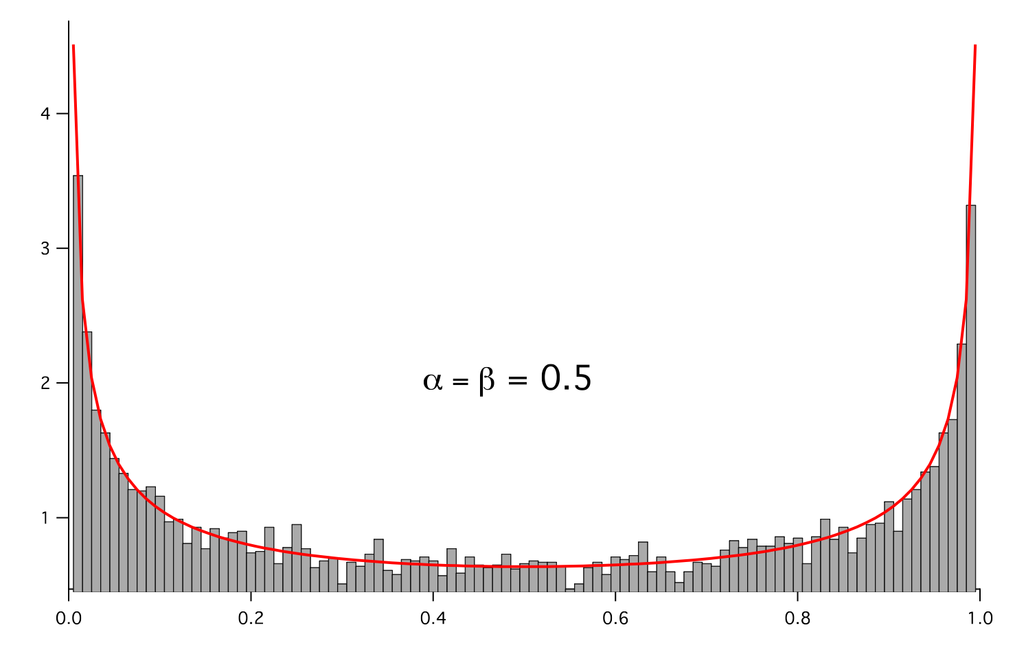
class fipy.variables.betaNoiseVariable.BetaNoiseVariable(mesh, alpha, beta, name='', hasOld=0)¶

Bases: fipy.variables.noiseVariable.NoiseVariable

Represents a beta distribution of random numbers with the probability distribution

$x^{\alpha - 1}\frac{\beta^\alpha e^{-\beta x}}{\Gamma(\alpha)}$

with a shape parameter $\alpha$ , a rate parameter $\beta$ , and $\Gamma(z) = \int_0^\infty t^{z - 1}e^{-t}\,dt$ .

Seed the random module for the sake of deterministic test results.

>>> from fipy import numerix
>>> numerix.random.seed(1)

We generate noise on a uniform cartesian mesh

>>> from fipy.variables.variable import Variable
>>> alpha = Variable()
>>> beta = Variable()
>>> from fipy.meshes import Grid2D
>>> noise = BetaNoiseVariable(mesh = Grid2D(nx = 100, ny = 100), alpha = alpha, beta = beta)

We histogram the root-volume-weighted noise distribution

>>> from fipy.variables.histogramVariable import HistogramVariable
>>> histogram = HistogramVariable(distribution = noise, dx = 0.01, nx = 100)

and compare to a Gaussian distribution

>>> from fipy.variables.cellVariable import CellVariable
>>> betadist = CellVariable(mesh = histogram.mesh)
>>> x = CellVariable(mesh=histogram.mesh, value=histogram.mesh.cellCenters[0])
>>> from scipy.special import gamma as Gamma 
>>> betadist = ((Gamma(alpha + beta) / (Gamma(alpha) * Gamma(beta))) 
...             * x**(alpha - 1) * (1 - x)**(beta - 1)) 

>>> if __name__ == '__main__':
...     from fipy import Viewer
...     viewer = Viewer(vars=noise, datamin=0, datamax=1)
...     histoplot = Viewer(vars=(histogram, betadist), 
...                        datamin=0, datamax=1.5)

>>> from fipy.tools.numerix import arange

>>> for a in arange(0.5,5,0.5):
...     alpha.value = a
...     for b in arange(0.5,5,0.5):
...         beta.value = b
...         if __name__ == '__main__':
...             import sys
...             print >>sys.stderr, "alpha: %g, beta: %g" % (alpha, beta)
...             viewer.plot()
...             histoplot.plot()

>>> print abs(noise.faceGrad.divergence.cellVolumeAverage) < 5e-15
1

Parameters :	mesh: The mesh on which to define the noise. alpha: The parameter $\alpha$ . beta: The parameter $\beta$ .

random()¶

`binaryOperatorVariable` Module¶

`cellToFaceVariable` Module¶

`cellVariable` Module¶

class fipy.variables.cellVariable.CellVariable(mesh, name='', value=0.0, rank=None, elementshape=None, unit=None, hasOld=0)¶

Bases: fipy.variables.meshVariable._MeshVariable

Represents the field of values of a variable on a Mesh.

A CellVariable can be pickled to persistent storage (disk) for later use:

>>> from fipy.meshes import Grid2D
>>> mesh = Grid2D(dx = 1., dy = 1., nx = 10, ny = 10)

>>> var = CellVariable(mesh = mesh, value = 1., hasOld = 1, name = 'test')
>>> x, y = mesh.cellCenters
>>> var.value = (x * y)

>>> from fipy.tools import dump        
>>> (f, filename) = dump.write(var, extension = '.gz')
>>> unPickledVar = dump.read(filename, f)

>>> print var.allclose(unPickledVar, atol = 1e-10, rtol = 1e-10)
1

arithmeticFaceValue¶

Returns a FaceVariable whose value corresponds to the arithmetic interpolation of the adjacent cells:

$\phi_f = (\phi_1 - \phi_2) \frac{d_{f2}}{d_{12}} + \phi_2$

>>> from fipy.meshes import Grid1D
>>> from fipy import numerix
>>> mesh = Grid1D(dx = (1., 1.))
>>> L = 1
>>> R = 2
>>> var = CellVariable(mesh = mesh, value = (L, R))
>>> faceValue = var.arithmeticFaceValue[mesh.interiorFaces.value]
>>> answer = (R - L) * (0.5 / 1.) + L
>>> print numerix.allclose(faceValue, answer, atol = 1e-10, rtol = 1e-10)
True

>>> mesh = Grid1D(dx = (2., 4.))
>>> var = CellVariable(mesh = mesh, value = (L, R))
>>> faceValue = var.arithmeticFaceValue[mesh.interiorFaces.value]
>>> answer = (R - L) * (1.0 / 3.0) + L
>>> print numerix.allclose(faceValue, answer, atol = 1e-10, rtol = 1e-10)
True

>>> mesh = Grid1D(dx = (10., 100.))
>>> var = CellVariable(mesh = mesh, value = (L, R))
>>> faceValue = var.arithmeticFaceValue[mesh.interiorFaces.value]
>>> answer = (R - L) * (5.0 / 55.0) + L
>>> print numerix.allclose(faceValue, answer, atol = 1e-10, rtol = 1e-10)
True

cellVolumeAverage¶

Return the cell-volume-weighted average of the CellVariable:

$<\phi>_\text{vol} = \frac{\sum_\text{cells} \phi_\text{cell} V_\text{cell}} {\sum_\text{cells} V_\text{cell}}$

>>> from fipy.meshes import Grid2D
>>> from fipy.variables.cellVariable import CellVariable
>>> mesh = Grid2D(nx = 3, ny = 1, dx = .5, dy = .1)
>>> var = CellVariable(value = (1, 2, 6), mesh = mesh)
>>> print var.cellVolumeAverage
3.0

constrain(value, where=None)¶

Constrains the CellVariable to value at a location specified by where.

>>> from fipy import *
>>> m = Grid1D(nx=3)
>>> v = CellVariable(mesh=m, value=m.cellCenters[0])
>>> v.constrain(0., where=m.facesLeft)
>>> v.faceGrad.constrain([1.], where=m.facesRight)
>>> print v.faceGrad
[[ 1.  1.  1.  1.]]
>>> print v.faceValue
[ 0.   1.   2.   2.5]

Changing the constraint changes the dependencies

>>> v.constrain(1., where=m.facesLeft)
>>> print v.faceGrad
[[-1.  1.  1.  1.]]
>>> print v.faceValue
[ 1.   1.   2.   2.5]

Constraints can be Variable

>>> c = Variable(0.)
>>> v.constrain(c, where=m.facesLeft)
>>> print v.faceGrad
[[ 1.  1.  1.  1.]]
>>> print v.faceValue
[ 0.   1.   2.   2.5]
>>> c.value = 1.
>>> print v.faceGrad
[[-1.  1.  1.  1.]]
>>> print v.faceValue
[ 1.   1.   2.   2.5]

Constraints can have a Variable mask.

>>> v = CellVariable(mesh=m)
>>> mask = FaceVariable(mesh=m, value=m.facesLeft)
>>> v.constrain(1., where=mask)
>>> print v.faceValue
[ 1.  0.  0.  0.]
>>> mask[:] = mask | m.facesRight
>>> print v.faceValue
[ 1.  0.  0.  1.]

copy()¶

faceGrad¶: Return $\nabla \phi$ as a rank-1 FaceVariable using differencing for the normal direction(second-order gradient).

faceGradAverage¶: Return $\nabla \phi$ as a rank-1 FaceVariable using averaging for the normal direction(second-order gradient)

faceValue¶

Returns a FaceVariable whose value corresponds to the arithmetic interpolation of the adjacent cells:

$\phi_f = (\phi_1 - \phi_2) \frac{d_{f2}}{d_{12}} + \phi_2$

>>> from fipy.meshes import Grid1D
>>> from fipy import numerix
>>> mesh = Grid1D(dx = (1., 1.))
>>> L = 1
>>> R = 2
>>> var = CellVariable(mesh = mesh, value = (L, R))
>>> faceValue = var.arithmeticFaceValue[mesh.interiorFaces.value]
>>> answer = (R - L) * (0.5 / 1.) + L
>>> print numerix.allclose(faceValue, answer, atol = 1e-10, rtol = 1e-10)
True

>>> mesh = Grid1D(dx = (2., 4.))
>>> var = CellVariable(mesh = mesh, value = (L, R))
>>> faceValue = var.arithmeticFaceValue[mesh.interiorFaces.value]
>>> answer = (R - L) * (1.0 / 3.0) + L
>>> print numerix.allclose(faceValue, answer, atol = 1e-10, rtol = 1e-10)
True

>>> mesh = Grid1D(dx = (10., 100.))
>>> var = CellVariable(mesh = mesh, value = (L, R))
>>> faceValue = var.arithmeticFaceValue[mesh.interiorFaces.value]
>>> answer = (R - L) * (5.0 / 55.0) + L
>>> print numerix.allclose(faceValue, answer, atol = 1e-10, rtol = 1e-10)
True

gaussGrad¶: Return $\frac{1}{V_P} \sum_f \vec{n} \phi_f A_f$ as a rank-1 CellVariable (first-order gradient).

getArithmeticFaceValue(*args, **kwds)¶: Deprecated since version 3.0: use the arithmeticFaceValue property instead

getCellVolumeAverage(*args, **kwds)¶: Deprecated since version 3.0: use the cellVolumeAverage property instead

getFaceGrad(*args, **kwds)¶: Deprecated since version 3.0: use the faceGrad property instead

getFaceGradAverage(*args, **kwds)¶: Deprecated since version 3.0: use the faceGradAverage property instead

getFaceValue(*args, **kwds)¶: Deprecated since version 3.0: use the arithmeticFaceValue property instead

getGaussGrad(*args, **kwds)¶: Deprecated since version 3.0: use the gaussGrad property instead

getGrad(*args, **kwds)¶: Deprecated since version 3.0: use the grad property instead

getHarmonicFaceValue(*args, **kwds)¶: Deprecated since version 3.0: use the harmonicFaceValue property instead

getLeastSquaresGrad(*args, **kwds)¶: Deprecated since version 3.0: use the leastSquaresGrad property instead

getMinmodFaceValue(*args, **kwds)¶: Deprecated since version 3.0: use the minmodFaceValue property instead

getOld(*args, **kwds)¶: Deprecated since version 3.0: use the old property instead

globalValue¶

Concatenate and return values from all processors

When running on a single processor, the result is identical to value.

grad¶: Return $\nabla \phi$ as a rank-1 CellVariable (first-order gradient).

harmonicFaceValue¶

Returns a FaceVariable whose value corresponds to the harmonic interpolation of the adjacent cells:

$\phi_f = \frac{\phi_1 \phi_2}{(\phi_2 - \phi_1) \frac{d_{f2}}{d_{12}} + \phi_1}$

>>> from fipy.meshes import Grid1D
>>> from fipy import numerix
>>> mesh = Grid1D(dx = (1., 1.))
>>> L = 1
>>> R = 2
>>> var = CellVariable(mesh = mesh, value = (L, R))
>>> faceValue = var.harmonicFaceValue[mesh.interiorFaces.value]
>>> answer = L * R / ((R - L) * (0.5 / 1.) + L)
>>> print numerix.allclose(faceValue, answer, atol = 1e-10, rtol = 1e-10)
True

>>> mesh = Grid1D(dx = (2., 4.))
>>> var = CellVariable(mesh = mesh, value = (L, R))
>>> faceValue = var.harmonicFaceValue[mesh.interiorFaces.value]
>>> answer = L * R / ((R - L) * (1.0 / 3.0) + L)
>>> print numerix.allclose(faceValue, answer, atol = 1e-10, rtol = 1e-10)
True

>>> mesh = Grid1D(dx = (10., 100.))
>>> var = CellVariable(mesh = mesh, value = (L, R))
>>> faceValue = var.harmonicFaceValue[mesh.interiorFaces.value]
>>> answer = L * R / ((R - L) * (5.0 / 55.0) + L)
>>> print numerix.allclose(faceValue, answer, atol = 1e-10, rtol = 1e-10)
True

leastSquaresGrad¶

Return $\nabla \phi$ , which is determined by solving for $\nabla \phi$ in the following matrix equation,

$\nabla \phi \cdot \sum_f d_{AP}^2 \vec{n}_{AP} \otimes \vec{n}_{AP} = \sum_f d_{AP}^2 \left( \vec{n} \cdot \nabla \phi \right)_{AP}$

The matrix equation is derived by minimizing the following least squares sum,

$F \left( \phi_x, \phi_y \right) = \sqrt{\sum_f \left( d_{AP} \vec{n}_{AP} \cdot \nabla \phi - d_{AP} \left( \vec{n}_{AP} \cdot \nabla \phi \right)_{AP} \right)^2 }$

Tests

>>> from fipy import Grid2D
>>> m = Grid2D(nx=2, ny=2, dx=0.1, dy=2.0)
>>> print numerix.allclose(CellVariable(mesh=m, value=(0,1,3,6)).leastSquaresGrad.globalValue, \
...                                     [[8.0, 8.0, 24.0, 24.0],
...                                      [1.2, 2.0, 1.2, 2.0]])
True

>>> from fipy import Grid1D
>>> print numerix.allclose(CellVariable(mesh=Grid1D(dx=(2.0, 1.0, 0.5)), 
...                                     value=(0, 1, 2)).leastSquaresGrad.globalValue, [[0.461538461538, 0.8, 1.2]])
True

minmodFaceValue¶

Returns a FaceVariable with a value that is the minimum of the absolute values of the adjacent cells. If the values are of opposite sign then the result is zero:

$\phi_f = \begin{cases} \phi_1& \text{when $|\phi_1| \le |\phi_2|$},\\ \phi_2& \text{when $|\phi_2| < |\phi_1|$},\\ 0 & \text{when $\phi1 \phi2 < 0$} \end{cases}$

>>> from fipy import *
>>> print CellVariable(mesh=Grid1D(nx=2), value=(1, 2)).minmodFaceValue
[1 1 2]
>>> print CellVariable(mesh=Grid1D(nx=2), value=(-1, -2)).minmodFaceValue
[-1 -1 -2]
>>> print CellVariable(mesh=Grid1D(nx=2), value=(-1, 2)).minmodFaceValue
[-1  0  2]

old¶

Return the values of the CellVariable from the previous solution sweep.

Combinations of CellVariable’s should also return old values.

>>> from fipy.meshes import Grid1D
>>> mesh = Grid1D(nx = 2)
>>> from fipy.variables.cellVariable import CellVariable
>>> var1 = CellVariable(mesh = mesh, value = (2, 3), hasOld = 1)
>>> var2 = CellVariable(mesh = mesh, value = (3, 4))
>>> v = var1 * var2
>>> print v
[ 6 12]
>>> var1.value = ((3,2))
>>> print v
[9 8]
>>> print v.old
[ 6 12]

The following small test is to correct for a bug when the operator does not just use variables.

>>> v1 = var1 * 3
>>> print v1
[9 6]
>>> print v1.old
[6 9]

release(constraint)¶

Remove constraint from self

>>> from fipy import *
>>> m = Grid1D(nx=3)
>>> v = CellVariable(mesh=m, value=m.cellCenters[0])
>>> c = Constraint(0., where=m.facesLeft)
>>> v.constrain(c)
>>> print v.faceValue
[ 0.   1.   2.   2.5]
>>> v.release(constraint=c)
>>> print v.faceValue
[ 0.5  1.   2.   2.5]

setValue(value, unit=None, where=None)¶

updateOld()¶

Set the values of the previous solution sweep to the current values.

>>> from fipy import *
>>> v = CellVariable(mesh=Grid1D(), hasOld=False)
>>> v.updateOld()
Traceback (most recent call last):
   ...
AssertionError: The updateOld method requires the CellVariable to have an old value. Set hasOld to True when instantiating the CellVariable.

`cellVolumeAverageVariable` Module¶

`constant` Module¶

`constraintMask` Module¶

`coupledCellVariable` Module¶

`distanceVariable` Module¶

class fipy.variables.distanceVariable.DistanceVariable(mesh, name='', value=0.0, unit=None, hasOld=0)¶

Bases: fipy.variables.cellVariable.CellVariable

A DistanceVariable object calculates $\phi$ so it satisfies,

$\abs{\nabla \phi} = 1$

using the fast marching method with an initial condition defined by the zero level set. The solution can either be first or second order.

Here we will define a few test cases. Firstly a 1D test case

>>> from fipy.meshes import Grid1D
>>> from fipy.tools import serialComm
>>> mesh = Grid1D(dx = .5, nx = 8, communicator=serialComm)
>>> from distanceVariable import DistanceVariable
>>> var = DistanceVariable(mesh = mesh, value = (-1., -1., -1., -1., 1., 1., 1., 1.))
>>> var.calcDistanceFunction() 
>>> answer = (-1.75, -1.25, -.75, -0.25, 0.25, 0.75, 1.25, 1.75)
>>> print var.allclose(answer) 
1

A 1D test case with very small dimensions.

>>> dx = 1e-10
>>> mesh = Grid1D(dx = dx, nx = 8, communicator=serialComm)
>>> var = DistanceVariable(mesh = mesh, value = (-1., -1., -1., -1., 1., 1., 1., 1.))
>>> var.calcDistanceFunction() 
>>> answer = numerix.arange(8) * dx - 3.5 * dx
>>> print var.allclose(answer) 
1

A 2D test case to test _calcTrialValue for a pathological case.

>>> dx = 1.
>>> dy = 2.
>>> from fipy.meshes import Grid2D
>>> mesh = Grid2D(dx = dx, dy = dy, nx = 2, ny = 3)
>>> var = DistanceVariable(mesh = mesh, value = (-1., 1., 1., 1., -1., 1.))

>>> var.calcDistanceFunction() 
>>> vbl = -dx * dy / numerix.sqrt(dx**2 + dy**2) / 2.
>>> vbr = dx / 2
>>> vml = dy / 2.
>>> crossProd = dx * dy
>>> dsq = dx**2 + dy**2
>>> top = vbr * dx**2 + vml * dy**2
>>> sqrt = crossProd**2 *(dsq - (vbr - vml)**2)
>>> sqrt = numerix.sqrt(max(sqrt, 0))
>>> vmr = (top + sqrt) / dsq
>>> answer = (vbl, vbr, vml, vmr, vbl, vbr)
>>> print var.allclose(answer) 
1

The extendVariable method solves the following equation for a given extensionVariable.

$\nabla u \cdot \nabla \phi = 0$

using the fast marching method with an initial condition defined at the zero level set.

>>> from fipy.variables.cellVariable import CellVariable
>>> mesh = Grid2D(dx = 1., dy = 1., nx = 2, ny = 2, communicator=serialComm)
>>> var = DistanceVariable(mesh = mesh, value = (-1., 1., 1., 1.))
>>> var.calcDistanceFunction() 
>>> extensionVar = CellVariable(mesh = mesh, value = (-1, .5, 2, -1))
>>> tmp = 1 / numerix.sqrt(2)
>>> print var.allclose((-tmp / 2, 0.5, 0.5, 0.5 + tmp)) 
1
>>> var.extendVariable(extensionVar, order=1) 
>>> print extensionVar.allclose((1.25, .5, 2, 1.25)) 
1
>>> mesh = Grid2D(dx = 1., dy = 1., nx = 3, ny = 3, communicator=serialComm)
>>> var = DistanceVariable(mesh = mesh, value = (-1., 1., 1.,
...                                               1., 1., 1.,
...                                               1., 1., 1.))
>>> var.calcDistanceFunction(order=1) 
>>> extensionVar = CellVariable(mesh = mesh, value = (-1., .5, -1.,
...                                                    2., -1., -1.,
...                                                   -1., -1., -1.))

>>> v1 = 0.5 + tmp
>>> v2 = 1.5
>>> tmp1 = (v1 + v2) / 2 + numerix.sqrt(2. - (v1 - v2)**2) / 2
>>> tmp2 = tmp1 + 1 / numerix.sqrt(2)
>>> print var.allclose((-tmp / 2, 0.5, 1.5, 0.5, 0.5 + tmp, 
...                      tmp1, 1.5, tmp1, tmp2)) 
1
>>> answer = (1.25, .5, .5, 2, 1.25, 0.9544, 2, 1.5456, 1.25)
>>> var.extendVariable(extensionVar, order=1) 
>>> print extensionVar.allclose(answer, rtol = 1e-4) 
1

Test case for a bug that occurs when initializing the distance variable at the interface. Currently it is assumed that adjacent cells that are opposite sign neighbors have perpendicular normal vectors. In fact the two closest cells could have opposite normals.

>>> mesh = Grid1D(dx = 1., nx = 3)
>>> var = DistanceVariable(mesh = mesh, value = (-1., 1., -1.))
>>> var.calcDistanceFunction() 
>>> print var.allclose((-0.5, 0.5, -0.5)) 
1

Testing second order. This example failed with Scikit-fmm.

>>> mesh = Grid2D(dx = 1., dy = 1., nx = 4, ny = 4, communicator=serialComm)
>>> var = DistanceVariable(mesh = mesh, value = (-1., -1., 1., 1.,
...                                               -1., -1., 1., 1.,
...                                               1., 1., 1., 1.,
...                                               1, 1, 1, 1))
>>> var.calcDistanceFunction(order=2) 
>>> answer = [-1.30473785, -0.5, 0.5, 1.49923009,
...           -0.5, -0.35355339, 0.5, 1.45118446,
...            0.5, 0.5, 0.97140452, 1.76215286,
...            1.49923009, 1.45118446, 1.76215286, 2.33721352]
>>> print numerix.allclose(var, answer, rtol=1e-9) 
True

** A test for a bug in both LSMLIB and Scikit-fmm **

The following test gives different result depending on whether LSMLIB or Scikit-fmm is used. There is a deeper problem that is related to this issue. When a value becomes “known” after previously being a “trial” value it updates its neighbors’ values. In a second order scheme the neighbors one step away also need to be updated (if the in between cell is “known” and the far cell is a “trial” cell), but are not in either package. By luck (due to trial values having the same value), the values calculated in Scikit-fmm for the following example are correct although an example that didn’t work for Scikit-fmm could also be constructed.

>>> mesh = Grid2D(dx = 1., dy = 1., nx = 4, ny = 4, communicator=serialComm)
>>> var = DistanceVariable(mesh = mesh, value = (-1., -1., -1., -1.,
...                                               1.,  1., -1., -1.,
...                                               1.,  1., -1., -1.,
...                                               1.,  1., -1., -1.))
>>> var.calcDistanceFunction(order=2) 
>>> var.calcDistanceFunction(order=2) 
>>> answer = [-0.5,        -0.58578644, -1.08578644, -1.85136395,
...            0.5,         0.29289322, -0.58578644, -1.54389939,
...            1.30473785,  0.5,        -0.5,        -1.5,
...            1.49547948,  0.5,        -0.5,        -1.5]

The 3rd and 7th element are different for LSMLIB. This is because the 15th element is not “known” when the “trial” value for the 7th element is calculated. Scikit-fmm calculates the values in a slightly different order so gets a seemingly better answer, but this is just chance.

>>> print numerix.allclose(var, answer, rtol=1e-9) 
True

Creates a distanceVariable object.

Parameters :	mesh: The mesh that defines the geometry of this variable. name: The name of the variable. value: The initial value. unit: the physical units of the variable hasOld: Whether the variable maintains an old value.

calcDistanceFunction(order=2)¶

Calculates the distanceVariable as a distance function.

Parameters :	order: The order of accuracy for the distance funtion calculation, either 1 or 2.

cellInterfaceAreas¶

Returns the length of the interface that crosses the cell

A simple 1D test:

>>> from fipy.meshes import Grid1D
>>> mesh = Grid1D(dx = 1., nx = 4)
>>> distanceVariable = DistanceVariable(mesh = mesh, 
...                                     value = (-1.5, -0.5, 0.5, 1.5))
>>> answer = CellVariable(mesh=mesh, value=(0, 0., 1., 0))
>>> print numerix.allclose(distanceVariable.cellInterfaceAreas, 
...                        answer)
True

A 2D test case:

>>> from fipy.meshes import Grid2D
>>> from fipy.variables.cellVariable import CellVariable
>>> mesh = Grid2D(dx = 1., dy = 1., nx = 3, ny = 3)
>>> distanceVariable = DistanceVariable(mesh = mesh, 
...                                     value = (1.5, 0.5, 1.5,
...                                              0.5,-0.5, 0.5,
...                                              1.5, 0.5, 1.5))
>>> answer = CellVariable(mesh=mesh,
...                       value=(0, 1, 0, 1, 0, 1, 0, 1, 0))
>>> print numerix.allclose(distanceVariable.cellInterfaceAreas, answer)
True

Another 2D test case:

>>> mesh = Grid2D(dx = .5, dy = .5, nx = 2, ny = 2)
>>> from fipy.variables.cellVariable import CellVariable
>>> distanceVariable = DistanceVariable(mesh = mesh, 
...                                     value = (-0.5, 0.5, 0.5, 1.5))
>>> answer = CellVariable(mesh=mesh,
...                       value=(0, numerix.sqrt(2) / 4,  numerix.sqrt(2) / 4, 0))
>>> print numerix.allclose(distanceVariable.cellInterfaceAreas, 
...                        answer)
True

Test to check that the circumfrence of a circle is, in fact, $2\pi r$ .

>>> mesh = Grid2D(dx = 0.05, dy = 0.05, nx = 20, ny = 20)
>>> r = 0.25
>>> x, y = mesh.cellCenters
>>> rad = numerix.sqrt((x - .5)**2 + (y - .5)**2) - r
>>> distanceVariable = DistanceVariable(mesh = mesh, value = rad)
>>> print numerix.allclose(distanceVariable.cellInterfaceAreas.sum(), 1.57984690073)
1

extendVariable(extensionVariable, order=2)¶

Calculates the extension of extensionVariable from the zero level set.

Parameters :	extensionVariable: The variable to extend from the zero level set.

getCellInterfaceAreas(*args, **kwds)¶: Deprecated since version 3.0: use the cellInterfaceAreas property instead

getLSMshape()¶

`exponentialNoiseVariable` Module¶

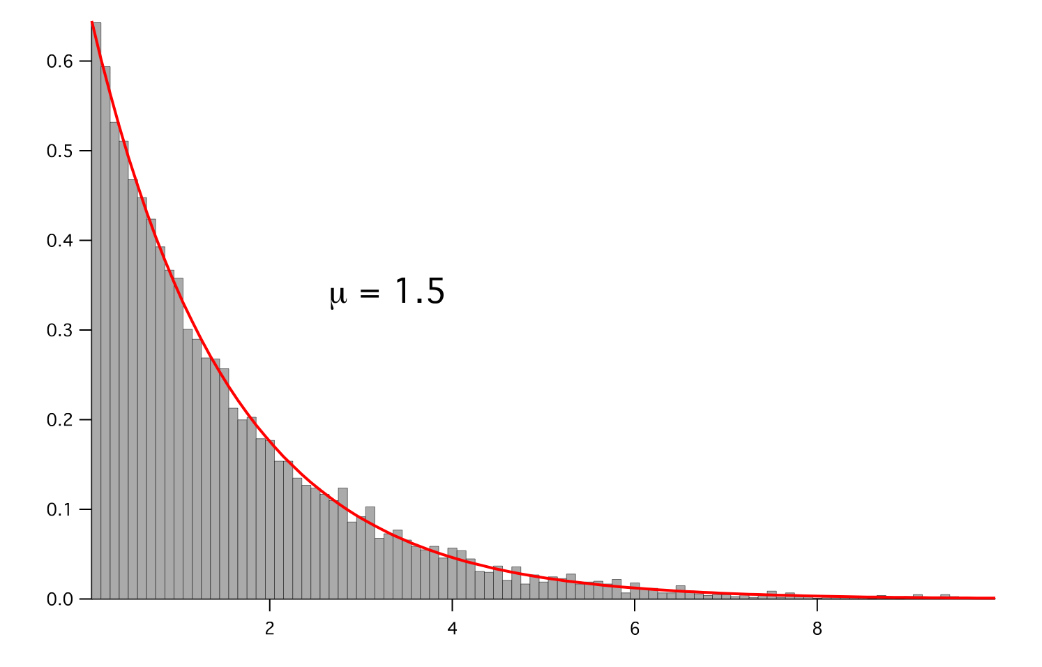
class fipy.variables.exponentialNoiseVariable.ExponentialNoiseVariable(mesh, mean=0.0, name='', hasOld=0)¶

Bases: fipy.variables.noiseVariable.NoiseVariable

Represents an exponential distribution of random numbers with the probability distribution

$\mu^{-1} e^{-\frac{x}{\mu}}$

with a mean parameter $\mu$ .

Seed the random module for the sake of deterministic test results.

>>> from fipy import numerix
>>> numerix.random.seed(1)

We generate noise on a uniform cartesian mesh

>>> from fipy.variables.variable import Variable
>>> mean = Variable()
>>> from fipy.meshes import Grid2D
>>> noise = ExponentialNoiseVariable(mesh = Grid2D(nx = 100, ny = 100), mean = mean)

We histogram the root-volume-weighted noise distribution

>>> from fipy.variables.histogramVariable import HistogramVariable
>>> histogram = HistogramVariable(distribution = noise, dx = 0.1, nx = 100)

and compare to a Gaussian distribution

>>> from fipy.variables.cellVariable import CellVariable
>>> expdist = CellVariable(mesh = histogram.mesh)
>>> x = histogram.mesh.cellCenters[0]

>>> if __name__ == '__main__':
...     from fipy import Viewer
...     viewer = Viewer(vars=noise, datamin=0, datamax=5)
...     histoplot = Viewer(vars=(histogram, expdist), 
...                        datamin=0, datamax=1.5)

>>> from fipy.tools.numerix import arange, exp

>>> for mu in arange(0.5,3,0.5):
...     mean.value = (mu)
...     expdist.value = ((1/mean)*exp(-x/mean))
...     if __name__ == '__main__':
...         import sys
...         print >>sys.stderr, "mean: %g" % mean
...         viewer.plot()
...         histoplot.plot()

>>> print abs(noise.faceGrad.divergence.cellVolumeAverage) < 5e-15
1

Parameters :	mesh: The mesh on which to define the noise. mean: The mean of the distribution $\mu$ .

random()¶

`faceGradContributionsVariable` Module¶

`faceGradVariable` Module¶

`faceVariable` Module¶

class fipy.variables.faceVariable.FaceVariable(mesh, name='', value=0.0, rank=None, elementshape=None, unit=None, cached=1)¶

Bases: fipy.variables.meshVariable._MeshVariable

Parameters :	mesh: the mesh that defines the geometry of this Variable name: the user-readable name of the Variable value: the initial value rank: the rank (number of dimensions) of each element of this Variable. Default: 0 elementshape: the shape of each element of this variable Default: rank * (mesh.dim,) unit: the physical units of the Variable

copy()¶

divergence¶

>>> from fipy.meshes import Grid2D
>>> from fipy.variables.cellVariable import CellVariable
>>> mesh = Grid2D(nx=3, ny=2)
>>> var = CellVariable(mesh=mesh, value=range(3*2))
>>> print var.faceGrad.divergence
[ 4.  3.  2. -2. -3. -4.]

getDivergence(*args, **kwds)¶: Deprecated since version 3.0: use the divergence property instead

globalValue¶

setValue(value, unit=None, where=None)¶

`gammaNoiseVariable` Module¶

class fipy.variables.gammaNoiseVariable.GammaNoiseVariable(mesh, shape, rate, name='', hasOld=0)¶

Bases: fipy.variables.noiseVariable.NoiseVariable

Represents a gamma distribution of random numbers with the probability distribution

$x^{\alpha - 1}\frac{\beta^\alpha e^{-\beta x}}{\Gamma(\alpha)}$

with a shape parameter $\alpha$ , a rate parameter $\beta$ , and $\Gamma(z) = \int_0^\infty t^{z - 1}e^{-t}\,dt$ .

Seed the random module for the sake of deterministic test results.

>>> from fipy import numerix
>>> numerix.random.seed(1)

We generate noise on a uniform cartesian mesh

>>> from fipy.variables.variable import Variable
>>> alpha = Variable()
>>> beta = Variable()
>>> from fipy.meshes import Grid2D
>>> noise = GammaNoiseVariable(mesh = Grid2D(nx = 100, ny = 100), shape = alpha, rate = beta)

We histogram the root-volume-weighted noise distribution

>>> from fipy.variables.histogramVariable import HistogramVariable
>>> histogram = HistogramVariable(distribution = noise, dx = 0.1, nx = 300)

and compare to a Gaussian distribution

>>> from fipy.variables.cellVariable import CellVariable
>>> x = CellVariable(mesh=histogram.mesh, value=histogram.mesh.cellCenters[0])
>>> from scipy.special import gamma as Gamma 
>>> from fipy.tools.numerix import exp
>>> gammadist = (x**(alpha - 1) * (beta**alpha * exp(-beta * x)) / Gamma(alpha)) 

>>> if __name__ == '__main__':
...     from fipy import Viewer
...     viewer = Viewer(vars=noise, datamin=0, datamax=30)
...     histoplot = Viewer(vars=(histogram, gammadist), 
...                        datamin=0, datamax=1)

>>> from fipy.tools.numerix import arange

>>> for shape in arange(1,8,1):
...     alpha.value = shape
...     for rate in arange(0.5,2.5,0.5):
...         beta.value = rate
...         if __name__ == '__main__':
...             import sys
...             print >>sys.stderr, "alpha: %g, beta: %g" % (alpha, beta)
...             viewer.plot()
...             histoplot.plot()

>>> print abs(noise.faceGrad.divergence.cellVolumeAverage) < 5e-15
1

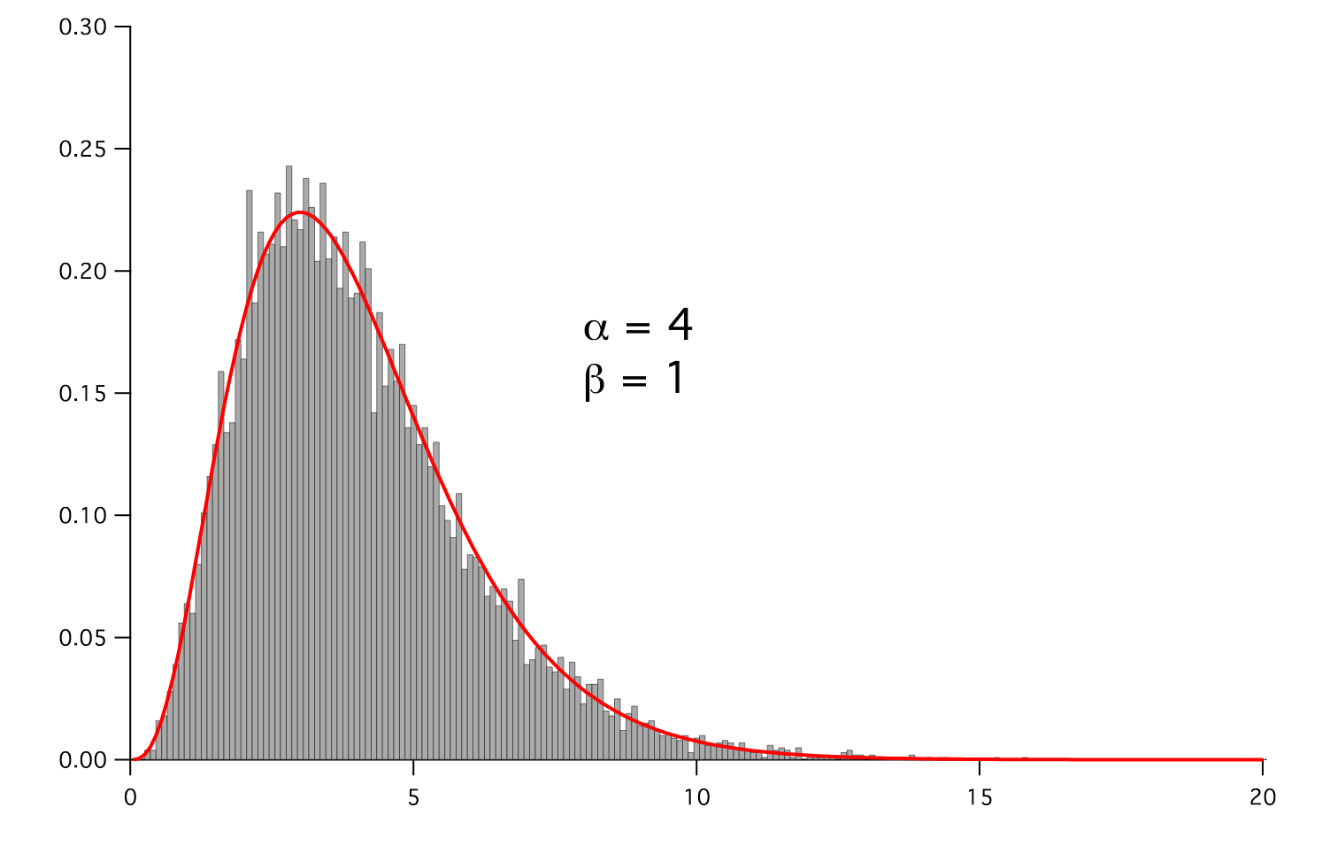
Parameters :	mesh: The mesh on which to define the noise. shape: The shape parameter, $\alpha$ . rate: The rate or inverse scale parameter, $\beta$ .

random()¶

`gaussCellGradVariable` Module¶

`gaussianNoiseVariable` Module¶

class fipy.variables.gaussianNoiseVariable.GaussianNoiseVariable(mesh, name='', mean=0.0, variance=1.0, hasOld=0)¶

Bases: fipy.variables.noiseVariable.NoiseVariable

Represents a normal (Gaussian) distribution of random numbers with mean $\mu$ and variance $\langle \eta(\vec{r}) \eta(\vec{r}\,') \rangle = \sigma^2$ , which has the probability distribution

$\frac{1}{\sigma\sqrt{2\pi}} \exp -\frac{(x - \mu)^2}{2\sigma^2}$

For example, the variance of thermal noise that is uncorrelated in space and time is often expressed as

$\left\langle \eta(\vec{r}, t) \eta(\vec{r}\,', t') \right\rangle = M k_B T \delta(\vec{r} - \vec{r}\,')\delta(t - t')$

which can be obtained with:

sigmaSqrd = Mobility * kBoltzmann * Temperature / (mesh.cellVolumes * timeStep)
GaussianNoiseVariable(mesh = mesh, variance = sigmaSqrd)

Note

If the time step will change as the simulation progresses, either through use of an adaptive iterator or by making manual changes at different stages, remember to declare timeStep as a Variable and to change its value with its setValue() method.

>>> import sys
>>> from fipy.tools.numerix import *

>>> mean = 0.
>>> variance = 4.

Seed the random module for the sake of deterministic test results.

>>> from fipy import numerix
>>> numerix.random.seed(3)

We generate noise on a non-uniform cartesian mesh with cell dimensions of $x^2$ and $y^3$ .

>>> from fipy.meshes import Grid2D
>>> mesh = Grid2D(dx = arange(0.1, 5., 0.1)**2, dy = arange(0.1, 3., 0.1)**3)
>>> from fipy.variables.cellVariable import CellVariable
>>> volumes = CellVariable(mesh=mesh,value=mesh.cellVolumes)
>>> noise = GaussianNoiseVariable(mesh = mesh, mean = mean, 
...                               variance = variance / volumes)

We histogram the root-volume-weighted noise distribution

>>> from fipy.variables.histogramVariable import HistogramVariable
>>> histogram = HistogramVariable(distribution = noise * sqrt(volumes), 
...                               dx = 0.1, nx = 600, offset = -30)

and compare to a Gaussian distribution

>>> gauss = CellVariable(mesh = histogram.mesh)
>>> x = histogram.mesh.cellCenters[0]
>>> gauss.value = ((1/(sqrt(variance * 2 * pi))) * exp(-(x - mean)**2 / (2 * variance)))

>>> if __name__ == '__main__':
...     from fipy.viewers import Viewer
...     viewer = Viewer(vars=noise, 
...                     datamin=-5, datamax=5)
...     histoplot = Viewer(vars=(histogram, gauss))

>>> for i in range(10):
...     noise.scramble()
...     if __name__ == '__main__':
...         viewer.plot()
...         histoplot.plot()

>>> print abs(noise.faceGrad.divergence.cellVolumeAverage) < 5e-15
1

Note that the noise exhibits larger amplitude in the small cells than in the large ones

but that the root-volume-weighted histogram is Gaussian.

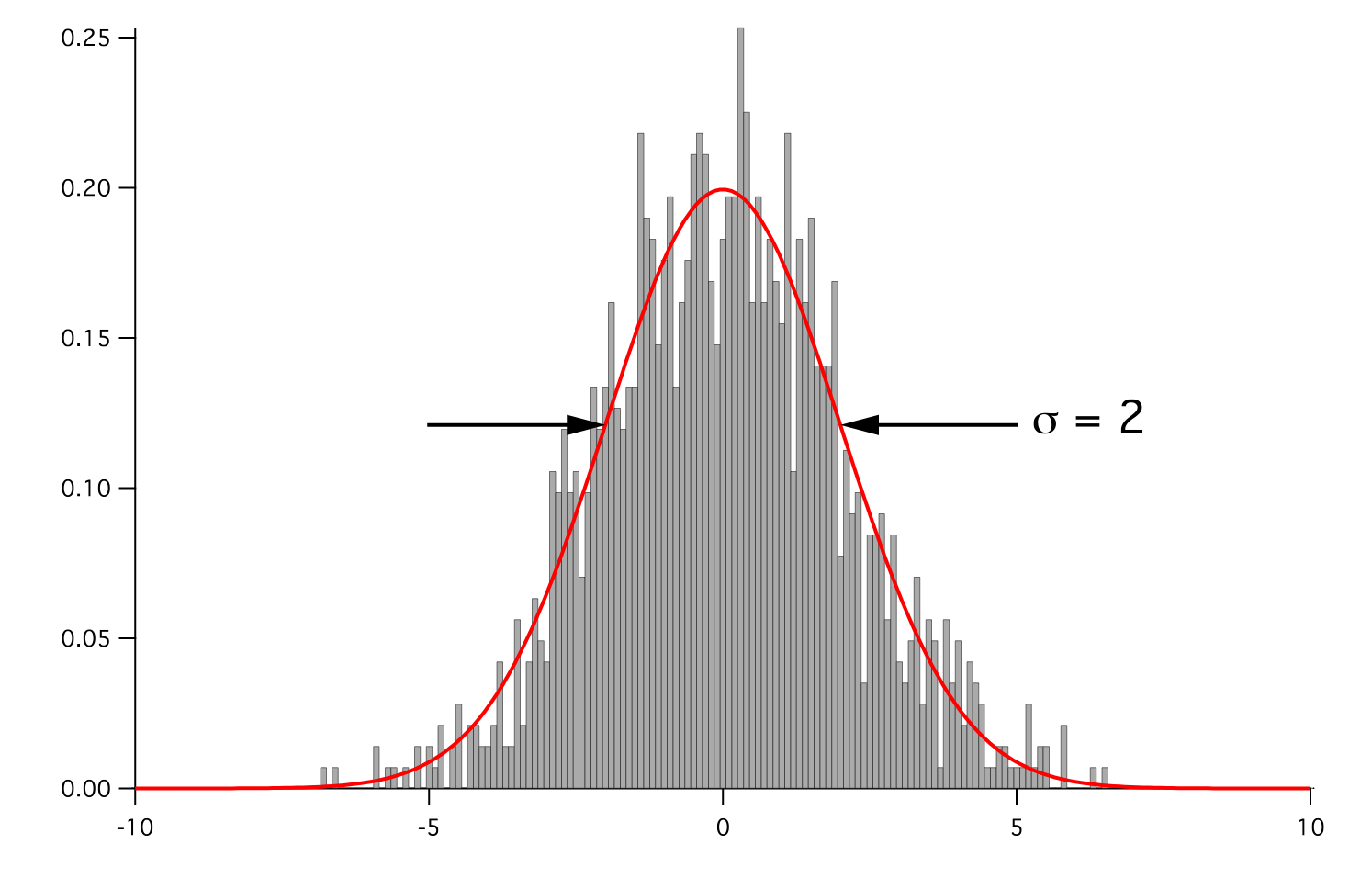
Parameters :	mesh: The mesh on which to define the noise. mean: The mean of the noise distrubution, $\mu$ . variance: The variance of the noise distribution, $\sigma^2$ .

parallelRandom()¶

`harmonicCellToFaceVariable` Module¶

`histogramVariable` Module¶

class fipy.variables.histogramVariable.HistogramVariable(distribution, dx=1.0, nx=None, offset=0.0)¶

Bases: fipy.variables.cellVariable.CellVariable

Produces a histogram of the values of the supplied distribution.

Parameters :	distribution: The collection of values to sample. dx: the bin size nx: the number of bins offset: the position of the first bin

`interfaceAreaVariable` Module¶

`interfaceFlagVariable` Module¶

`leastSquaresCellGradVariable` Module¶

`levelSetDiffusionVariable` Module¶

`meshVariable` Module¶

`minmodCellToFaceVariable` Module¶

`modCellGradVariable` Module¶

`modCellToFaceVariable` Module¶

`modFaceGradVariable` Module¶

`modPhysicalField` Module¶

`modularVariable` Module¶

class fipy.variables.modularVariable.ModularVariable(mesh, name='', value=0.0, rank=None, elementshape=None, unit=None, hasOld=0)¶

Bases: fipy.variables.cellVariable.CellVariable

The ModularVariable defines a variable that exisits on the circle between $-\pi$ and $\pi$

The following examples show how ModularVariable works. When subtracting the answer wraps back around the circle.

>>> from fipy.meshes import Grid1D
>>> mesh = Grid1D(nx = 2)
>>> from fipy.tools import numerix
>>> pi = numerix.pi
>>> v1 = ModularVariable(mesh = mesh, value = (2*pi/3, -2*pi/3))
>>> v2 = ModularVariable(mesh = mesh, value = -2*pi/3)
>>> print numerix.allclose(v2 - v1, (2*pi/3, 0))
1

Obtaining the arithmetic face value.

>>> print numerix.allclose(v1.arithmeticFaceValue, (2*pi/3, pi, -2*pi/3))
1

Obtaining the gradient.

>>> print numerix.allclose(v1.grad, ((pi/3, pi/3),))
1

Obtaining the gradient at the faces.

>>> print numerix.allclose(v1.faceGrad, ((0, 2*pi/3, 0),))
1

Obtaining the gradient at the faces but without modular arithmetic.

>>> print numerix.allclose(v1.faceGradNoMod, ((0, -4*pi/3, 0),))
1

arithmeticFaceValue¶

Returns a FaceVariable whose value corresponds to the arithmetic interpolation of the adjacent cells:

$\phi_f = (\phi_1 - \phi_2) \frac{d_{f2}}{d_{12}} + \phi_2$

Adjusted for a ModularVariable

faceGrad¶: Return $\nabla \phi$ as a rank-1 FaceVariable (second-order gradient). Adjusted for a ModularVariable

faceGradNoMod¶: Return $\nabla \phi$ as a rank-1 FaceVariable (second-order gradient). Not adjusted for a ModularVariable

getFaceGradNoMod(*args, **kwds)¶: Deprecated since version 3.0: use the faceGradNoMod property instead

grad¶: Return $\nabla \phi$ as a rank-1 CellVariable (first-order gradient). Adjusted for a ModularVariable

updateOld()¶

Set the values of the previous solution sweep to the current values. Test case due to bug.

>>> from fipy.meshes import Grid1D
>>> mesh = Grid1D(nx = 1)
>>> var = ModularVariable(mesh=mesh, value=1., hasOld=1)
>>> var.updateOld()
>>> var[:] = 2
>>> answer = CellVariable(mesh=mesh, value=1.)
>>> print var.old.allclose(answer)
True

`noiseVariable` Module¶

class fipy.variables.noiseVariable.NoiseVariable(mesh, name='', hasOld=0)¶

Bases: fipy.variables.cellVariable.CellVariable

Attention

This class is abstract. Always create one of its subclasses.

A generic base class for sources of noise distributed over the cells of a mesh.

In the event that the noise should be conserved, use:

<Specific>NoiseVariable(...).faceGrad.divergence

The seed() and get_seed() functions of the fipy.tools.numerix.random module can be set and query the random number generated used by all NoiseVariable objects.

copy()¶: Copy the value of the NoiseVariable to a static CellVariable.

parallelRandom()¶

random()¶

scramble()¶: Generate a new random distribution.

`operatorVariable` Module¶

`scharfetterGummelFaceVariable` Module¶

class fipy.variables.scharfetterGummelFaceVariable.ScharfetterGummelFaceVariable(var, boundaryConditions=())¶: Bases: fipy.variables.cellToFaceVariable._CellToFaceVariable

`surfactantConvectionVariable` Module¶

class fipy.variables.surfactantConvectionVariable.SurfactantConvectionVariable(distanceVar)¶

Bases: fipy.variables.faceVariable.FaceVariable

Convection coefficient for the ConservativeSurfactantEquation. The coeff only has a value for a negative distanceVar.

Simple one dimensional test:

>>> from fipy.variables.cellVariable import CellVariable
>>> from fipy.meshes import Grid2D
>>> mesh = Grid2D(nx = 3, ny = 1, dx = 1., dy = 1.)
>>> from fipy.variables.distanceVariable import DistanceVariable
>>> distanceVar = DistanceVariable(mesh, value = (-.5, .5, 1.5))
>>> ## answer = numerix.zeros((2, mesh.numberOfFaces),'d')
>>> answer = FaceVariable(mesh=mesh, rank=1, value=0.).globalValue
>>> answer[0,7] = -1
>>> print numerix.allclose(SurfactantConvectionVariable(distanceVar).globalValue, answer)
True

Change the dimensions:

>>> mesh = Grid2D(nx = 3, ny = 1, dx = .5, dy = .25)
>>> distanceVar = DistanceVariable(mesh, value = (-.25, .25, .75))
>>> answer[0,7] = -.5
>>> print numerix.allclose(SurfactantConvectionVariable(distanceVar).globalValue, answer)
True

Two dimensional example:

>>> mesh = Grid2D(nx = 2, ny = 2, dx = 1., dy = 1.)
>>> distanceVar = DistanceVariable(mesh, value = (-1.5, -.5, -.5, .5))
 >>> answer = FaceVariable(mesh=mesh, rank=1, value=0.).globalValue
>>> answer[1,2] = -.5
>>> answer[1,3] = -1
>>> answer[0,7] = -.5
>>> answer[0,10] = -1
>>> print numerix.allclose(SurfactantConvectionVariable(distanceVar).globalValue, answer)
True

Larger grid:

>>> mesh = Grid2D(nx = 3, ny = 3, dx = 1., dy = 1.)
>>> distanceVar = DistanceVariable(mesh, value = (1.5, .5 , 1.5,
...                                           .5 , -.5, .5 ,
...                                           1.5, .5 , 1.5))
 >>> answer = FaceVariable(mesh=mesh, rank=1, value=0.).globalValue
>>> answer[1,4] = .25
>>> answer[1,7] = -.25
>>> answer[0,17] = .25
>>> answer[0,18] = -.25
>>> print numerix.allclose(SurfactantConvectionVariable(distanceVar).globalValue, answer)
True

`surfactantVariable` Module¶

class fipy.variables.surfactantVariable.SurfactantVariable(value=0.0, distanceVar=None, name='surfactant variable', hasOld=False)¶

Bases: fipy.variables.cellVariable.CellVariable

The SurfactantVariable maintains a conserved volumetric concentration on cells adjacent to, but in front of, the interface. The value argument corresponds to the initial concentration of surfactant on the interface (moles divided by area). The value held by the SurfactantVariable is actually a volume density (moles divided by volume).

A simple 1D test:

>>> from fipy.meshes import Grid1D
>>> mesh = Grid1D(dx = 1., nx = 4)
>>> from fipy.variables.distanceVariable import DistanceVariable
>>> distanceVariable = DistanceVariable(mesh = mesh, 
...                                     value = (-1.5, -0.5, 0.5, 941.5))
>>> surfactantVariable = SurfactantVariable(value = 1, 
...                                         distanceVar = distanceVariable)
>>> print numerix.allclose(surfactantVariable, (0, 0., 1., 0))
1

A 2D test case:

>>> from fipy.meshes import Grid2D
>>> mesh = Grid2D(dx = 1., dy = 1., nx = 3, ny = 3)
>>> distanceVariable = DistanceVariable(mesh = mesh,
...                                     value = (1.5, 0.5, 1.5,
...                                              0.5,-0.5, 0.5,
...                                              1.5, 0.5, 1.5))
>>> surfactantVariable = SurfactantVariable(value = 1, 
...                                         distanceVar = distanceVariable)
>>> print numerix.allclose(surfactantVariable, (0, 1, 0, 1, 0, 1, 0, 1, 0))
1

Another 2D test case:

>>> mesh = Grid2D(dx = .5, dy = .5, nx = 2, ny = 2)
>>> distanceVariable = DistanceVariable(mesh = mesh, 
...                                     value = (-0.5, 0.5, 0.5, 1.5))
>>> surfactantVariable = SurfactantVariable(value = 1, 
...                                         distanceVar = distanceVariable)
>>> print numerix.allclose(surfactantVariable, 
...                  (0, numerix.sqrt(2), numerix.sqrt(2), 0))
1

Parameters :	value: The initial value. distanceVar: A DistanceVariable object. name: The name of the variable.

copy()¶

getInterfaceVar(*args, **kwds)¶: Deprecated since version 3.0: use the interfaceVar property instead

interfaceVar¶: Returns the SurfactantVariable rendered as an _InterfaceSurfactantVariable which evaluates the surfactant concentration as an area concentration the interface rather than a volumetric concentration.

`test` Module¶

Test numeric implementation of the mesh

`unaryOperatorVariable` Module¶

`uniformNoiseVariable` Module¶

class fipy.variables.uniformNoiseVariable.UniformNoiseVariable(mesh, name='', minimum=0.0, maximum=1.0, hasOld=0)¶

Bases: fipy.variables.noiseVariable.NoiseVariable

Represents a uniform distribution of random numbers.

We generate noise on a uniform cartesian mesh

>>> from fipy.meshes import Grid2D
>>> noise = UniformNoiseVariable(mesh=Grid2D(nx=100, ny=100))

and histogram the noise

>>> from fipy.variables.histogramVariable import HistogramVariable
>>> histogram = HistogramVariable(distribution=noise, dx=0.01, nx=120, offset=-.1)

>>> if __name__ == '__main__':
...     from fipy import Viewer
...     viewer = Viewer(vars=noise, 
...                     datamin=0, datamax=1)
...     histoplot = Viewer(vars=histogram)

>>> for i in range(10):
...     noise.scramble()
...     if __name__ == '__main__':
...         viewer.plot()
...         histoplot.plot()

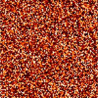
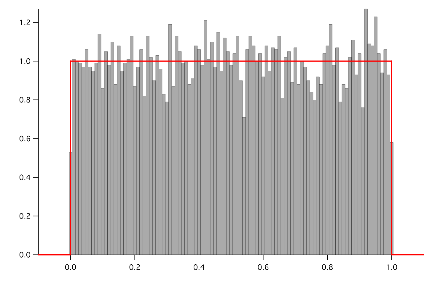
Parameters :	mesh: The mesh on which to define the noise. minimum: The minimum (not-inclusive) value of the distribution. maximum: The maximum (not-inclusive) value of the distribution.

random()¶

`variable` Module¶

class fipy.variables.variable.Variable(value=0.0, unit=None, array=None, name='', cached=1)¶

Bases: object

Lazily evaluated quantity with units.

Using a Variable in a mathematical expression will create an automatic dependency Variable, e.g.,

>>> a = Variable(value=3)
>>> b = 4 * a
>>> b
(Variable(value=array(3)) * 4)
>>> b()
12

Changes to the value of a Variable will automatically trigger changes in any dependent Variable objects

>>> a.setValue(5)
>>> b
(Variable(value=array(5)) * 4)
>>> print b()
20

Create a Variable.

>>> Variable(value=3)
Variable(value=array(3))
>>> Variable(value=3, unit="m")
Variable(value=PhysicalField(3,'m'))
>>> Variable(value=3, unit="m", array=numerix.zeros((3,2), 'l'))
Variable(value=PhysicalField(array([[3, 3],
       [3, 3],
       [3, 3]]),'m'))

Parameters :	value: the initial value unit: the physical units of the Variable array: the storage array for the Variable name: the user-readable name of the Variable cached: whether to cache or always recalculate the value

all(axis=None)¶

>>> print Variable(value=(0, 0, 1, 1)).all()
0
>>> print Variable(value=(1, 1, 1, 1)).all()
1

allclose(other, rtol=1e-05, atol=1e-08)¶

>>> var = Variable((1, 1))
   >>> print var.allclose((1, 1))
   1
   >>> print var.allclose((1,))
   1

The following test is to check that the system does not run out of memory.

>>> from fipy.tools import numerix
>>> var = Variable(numerix.ones(10000))
>>> print var.allclose(numerix.zeros(10000, 'l'))
False

allequal(other)¶

any(axis=None)¶

>>> print Variable(value=0).any()
0
>>> print Variable(value=(0, 0, 1, 1)).any()
1

arccos(*args, **kwds)¶: Deprecated since version 3.0: use numerix.arccos() instead

arccosh(*args, **kwds)¶: Deprecated since version 3.0: use numerix.arccosh() instead

arcsin(*args, **kwds)¶: Deprecated since version 3.0: use numerix.arcsin() instead

arcsinh(*args, **kwds)¶: Deprecated since version 3.0: use numerix.arcsinh() instead

arctan(*args, **kwds)¶: Deprecated since version 3.0: use numerix.arctan() instead

arctan2(*args, **kwds)¶: Deprecated since version 3.0: use numerix.arctan2() instead

arctanh(*args, **kwds)¶: Deprecated since version 3.0: use numerix.arctanh() instead

cacheMe(recursive=False)¶

ceil(*args, **kwds)¶: Deprecated since version 3.0: use numerix.ceil() instead

conjugate(*args, **kwds)¶: Deprecated since version 3.0: use numerix.conjugate() instead

constrain(value, where=None)¶

Constrain the Variable to have a value at an index or mask location specified by where.

>>> v = Variable((0,1,2,3))
>>> v.constrain(2, numerix.array((True, False, False, False)))
>>> print v
[2 1 2 3]
>>> v[:] = 10
>>> print v
[ 2 10 10 10]
>>> v.constrain(5, numerix.array((False, False, True, False)))
>>> print v
[ 2 10  5 10]
>>> v[:] = 6
>>> print v
[2 6 5 6]
>>> v.constrain(8)
>>> print v
[8 8 8 8]
>>> v[:] = 10
>>> print v
[8 8 8 8]
>>> del v.constraints[2]
>>> print v
[ 2 10  5 10]

>>> from fipy.variables.cellVariable import CellVariable
>>> from fipy.meshes import Grid2D
>>> m = Grid2D(nx=2, ny=2)
>>> x, y = m.cellCenters
>>> v = CellVariable(mesh=m, rank=1, value=(x, y))
>>> v.constrain(((0.,), (-1.,)), where=m.facesLeft)
>>> print v.faceValue
[[ 0.5  1.5  0.5  1.5  0.5  1.5  0.   1.   1.5  0.   1.   1.5]
 [ 0.5  0.5  1.   1.   1.5  1.5 -1.   0.5  0.5 -1.   1.5  1.5]]

Parameters :	value: the value of the constraint where: the constraint mask or index specifying the location of the constraint

constraints¶

copy()¶

Make an duplicate of the Variable

>>> a = Variable(value=3)
>>> b = a.copy()
>>> b
Variable(value=array(3))

The duplicate will not reflect changes made to the original

>>> a.setValue(5)
>>> b
Variable(value=array(3))

Check that this works for arrays.

>>> a = Variable(value=numerix.array((0,1,2)))
>>> b = a.copy()
>>> b
Variable(value=array([0, 1, 2]))
>>> a[1] = 3
>>> b
Variable(value=array([0, 1, 2]))

cos(*args, **kwds)¶: Deprecated since version 3.0: use numerix.cos() instead

cosh(*args, **kwds)¶: Deprecated since version 3.0: use numerix.cosh() instead

dontCacheMe(recursive=False)¶

dot(other, opShape=None, operatorClass=None, axis=0)¶

exp(*args, **kwds)¶: Deprecated since version 3.0: use numerix.exp() instead

floor(*args, **kwds)¶: Deprecated since version 3.0: use numerix.floor() instead

getMag(*args, **kwds)¶: Deprecated since version 3.0: use the mag property instead

getName(*args, **kwds)¶: Deprecated since version 3.0: use the name property instead

getNumericValue(*args, **kwds)¶: Deprecated since version 3.0: use the numericValue property instead

getShape(*args, **kwds)¶: Deprecated since version 3.0: use the shape property instead

getSubscribedVariables(*args, **kwds)¶: Deprecated since version 3.0: use the subscribedVariables property instead

getUnit(*args, **kwds)¶: Deprecated since version 3.0: use the unit property instead

getValue(*args, **kwds)¶: Deprecated since version 3.0: use the value property instead

getsctype(default=None)¶

Returns the Numpy sctype of the underlying array.

>>> Variable(1).getsctype() == numerix.NUMERIX.obj2sctype(numerix.array(1))
True
>>> Variable(1.).getsctype() == numerix.NUMERIX.obj2sctype(numerix.array(1.))
True
>>> Variable((1,1.)).getsctype() == numerix.NUMERIX.obj2sctype(numerix.array((1., 1.)))
True

inBaseUnits()¶

Return the value of the Variable with all units reduced to their base SI elements.

>>> e = Variable(value="2.7 Hartree*Nav")
>>> print e.inBaseUnits().allclose("7088849.01085 kg*m**2/s**2/mol")
1

inUnitsOf(*units)¶

Returns one or more Variable objects that express the same physical quantity in different units. The units are specified by strings containing their names. The units must be compatible with the unit of the object. If one unit is specified, the return value is a single Variable.

>>> freeze = Variable('0 degC')
>>> print freeze.inUnitsOf('degF').allclose("32.0 degF")
1

If several units are specified, the return value is a tuple of Variable instances with with one element per unit such that the sum of all quantities in the tuple equals the the original quantity and all the values except for the last one are integers. This is used to convert to irregular unit systems like hour/minute/second. The original object will not be changed.

>>> t = Variable(value=314159., unit='s')
>>> print numerix.allclose([e.allclose(v) for (e, v) in zip(t.inUnitsOf('d','h','min','s'),
...                                                         ['3.0 d', '15.0 h', '15.0 min', '59.0 s'])], 
...                        True)
1

itemset(value)¶

itemsize¶

log(*args, **kwds)¶: Deprecated since version 3.0: use numerix.log() instead

log10(*args, **kwds)¶: Deprecated since version 3.0: use numerix.log10() instead

mag¶

max(axis=None)¶

min(axis=None)¶

name¶

numericValue¶

put(indices, value)¶

ravel()¶

release(constraint)¶

Remove constraint from self

>>> v = Variable((0,1,2,3))
>>> v.constrain(2, numerix.array((True, False, False, False)))
>>> v[:] = 10
>>> from fipy.boundaryConditions.constraint import Constraint
>>> c1 = Constraint(5, numerix.array((False, False, True, False)))
>>> v.constrain(c1)
>>> v[:] = 6
>>> v.constrain(8)
>>> v[:] = 10
>>> del v.constraints[2]
>>> v.release(constraint=c1)
>>> print v
[ 2 10 10 10]

reshape(*args, **kwds)¶: Deprecated since version 3.0: use numerix.reshape() instead

setName(*args, **kwds)¶: Deprecated since version 3.0: use the name property instead

setUnit(*args, **kwds)¶: Deprecated since version 3.0: use the unit property instead

setValue(value, unit=None, where=None)¶

Set the value of the Variable. Can take a masked array.

>>> a = Variable((1,2,3))
>>> a.setValue(5, where=(1, 0, 1))
>>> print a
[5 2 5]

>>> b = Variable((4,5,6))
>>> a.setValue(b, where=(1, 0, 1))
>>> print a
[4 2 6]
>>> print b
[4 5 6]
>>> a.value = 3
>>> print a
[3 3 3]

>>> b = numerix.array((3,4,5))
>>> a.value = b
>>> a[:] = 1
>>> print b
[3 4 5]

>>> a.setValue((4,5,6), where=(1, 0)) 
Traceback (most recent call last):
    ....
ValueError: shape mismatch: objects cannot be broadcast to a single shape

shape¶

Tuple of array dimensions.

>>> Variable(value=3).shape
()
>>> Variable(value=(3,)).shape
(1,)
>>> Variable(value=(3,4)).shape
(2,)

>>> Variable(value="3 m").shape
()
>>> Variable(value=(3,), unit="m").shape
(1,)
>>> Variable(value=(3,4), unit="m").shape
(2,)

sign(*args, **kwds)¶: Deprecated since version 3.0: use numerix.sign() instead

sin(*args, **kwds)¶: Deprecated since version 3.0: use numerix.sin() instead

sinh(*args, **kwds)¶: Deprecated since version 3.0: use numerix.sinh() instead

sqrt(*args, **kwds)¶

Deprecated since version 3.0: use numerix.sqrt() instead

>>> from fipy.meshes import Grid1D
>>> mesh= Grid1D(nx=3)

>>> from fipy.variables.cellVariable import CellVariable
>>> var = CellVariable(mesh=mesh, value=((0., 2., 3.),), rank=1)
>>> print (var.dot(var)).sqrt()
[ 0.  2.  3.]

subscribedVariables¶

sum(axis=None)¶

take(ids, axis=0)¶

tan(*args, **kwds)¶: Deprecated since version 3.0: use numerix.tan() instead

tanh(*args, **kwds)¶: Deprecated since version 3.0: use numerix.tanh() instead

tostring(max_line_width=75, precision=8, suppress_small=False, separator=' ')¶

unit¶

Return the unit object of self.

>>> Variable(value="1 m").unit
<PhysicalUnit m>

value¶

“Evaluate” the Variable and return its value (longhand)

>>> a = Variable(value=3)
>>> print a.value
3
>>> b = a + 4
>>> b
(Variable(value=array(3)) + 4)
>>> b.value
7

Navigation

Table Of Contents

Previous topic

Next topic

This Page

Quick search

Contact

variables Package¶