examples.diffusion.mesh1D¶

Solve a one-dimensional diffusion equation under different conditions.

To run this example from the base FiPy directory, type:

$ python examples/diffusion/mesh1D.py

at the command line. Different stages of the example should be displayed, along with prompting messages in the terminal.

This example takes the user through assembling a simple problem with FiPy. It describes different approaches to a 1D diffusion problem with constant diffusivity and fixed value boundary conditions such that,

(1)¶ $\frac{\partial \phi}{\partial t} = D \nabla^2 \phi.$

The first step is to define a one dimensional domain with 50 solution points. The Grid1D object represents a linear structured grid. The parameter dx refers to the grid spacing (set to unity here).

>>> from fipy import Variable, FaceVariable, CellVariable, Grid1D, ExplicitDiffusionTerm, TransientTerm, DiffusionTerm, Viewer
>>> from fipy.tools import numerix

>>> nx = 50
>>> dx = 1.
>>> mesh = Grid1D(nx=nx, dx=dx)

FiPy solves all equations at the centers of the cells of the mesh. We thus need a CellVariable object to hold the values of the solution, with the initial condition $\phi = 0$ at $t = 0$ ,

>>> phi = CellVariable(name="solution variable",
...                    mesh=mesh,
...                    value=0.)

We’ll let

>>> D = 1.

for now.

The boundary conditions

$\phi = \begin{cases} 0& \text{at $x = 1$,} \\ 1& \text{at $x = 0$.} \end{cases}$

are formed with a value

>>> valueLeft = 1
>>> valueRight = 0

and a set of faces over which they apply.

Note

Only faces around the exterior of the mesh can be used for boundary conditions.

For example, here the exterior faces on the left of the domain are extracted by mesh.facesLeft. The boundary conditions are applied using phi. constrain() with these faces and a value (valueLeft).

>>> phi.constrain(valueRight, mesh.facesRight)
>>> phi.constrain(valueLeft, mesh.facesLeft)

Note

If no boundary conditions are specified on exterior faces, the default boundary condition is no-flux, $\vec{n} \cdot (D \nabla \phi) \rvert_\text{someFaces} = 0$ .

If you have ever tried to numerically solve Eq. (1), you most likely attempted “explicit finite differencing” with code something like:

for step in range(steps):
    for j in range(cells):
        phi_new[j] = phi_old[j] \
          + (D * dt / dx**2) * (phi_old[j+1] - 2 * phi_old[j] + phi_old[j-1])
    time += dt

plus additional code for the boundary conditions. In FiPy, you would write

>>> eqX = TransientTerm() == ExplicitDiffusionTerm(coeff=D)

The largest stable timestep that can be taken for this explicit 1D diffusion problem is $\Delta t \le \Delta x^2 / (2 D)$ .

We limit our steps to 90% of that value for good measure

>>> timeStepDuration = 0.9 * dx**2 / (2 * D)
>>> steps = 100

If we’re running interactively, we’ll want to view the result, but not if this example is being run automatically as a test. We accomplish this by having Python check if this script is the “__main__” script, which will only be true if we explicitly launched it and not if it has been imported by another script such as the automatic tester. The factory function Viewer() returns a suitable viewer depending on available viewers and the dimension of the mesh.

>>> phiAnalytical = CellVariable(name="analytical value",
...                              mesh=mesh)

>>> if __name__ == '__main__':
...     viewer = Viewer(vars=(phi, phiAnalytical),
...                     datamin=0., datamax=1.)
...     viewer.plot()

In a semi-infinite domain, the analytical solution for this transient diffusion problem is given by $\phi = 1 - \erf(x/2\sqrt{D t})$ . If the SciPy library is available, the result is tested against the expected profile:

>>> x = mesh.cellCenters[0]
>>> t = timeStepDuration * steps

>>> try:
...     from scipy.special import erf 
...     phiAnalytical.setValue(1 - erf(x / (2 * numerix.sqrt(D * t)))) 
... except ImportError:
...     print("The SciPy library is not available to test the solution to \
... the transient diffusion equation")

We then solve the equation by repeatedly looping in time:

>>> from builtins import range
>>> for step in range(steps):
...     eqX.solve(var=phi,
...               dt=timeStepDuration)
...     if __name__ == '__main__':
...         viewer.plot()

>>> print(phi.allclose(phiAnalytical, atol = 7e-4)) 
1

>>> from fipy import input
>>> if __name__ == '__main__':
...     input("Explicit transient diffusion. Press <return> to proceed...")

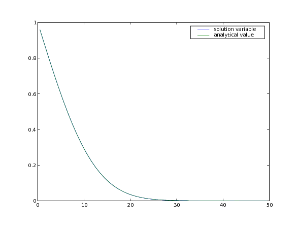
solution to diffusion problem evolved by explicit time steps

Although explicit finite differences are easy to program, we have just seen that this 1D transient diffusion problem is limited to taking rather small time steps. If, instead, we represent Eq. (1) as:

phi_new[j] = phi_old[j] \
  + (D * dt / dx**2) * (phi_new[j+1] - 2 * phi_new[j] + phi_new[j-1])

it is possible to take much larger time steps. Because phi_new appears on both the left and right sides of the equation, this form is called “implicit”. In general, the “implicit” representation is much more difficult to program than the “explicit” form that we just used, but in FiPy, all that is needed is to write

>>> eqI = TransientTerm() == DiffusionTerm(coeff=D)

reset the problem

>>> phi.setValue(valueRight)

and rerun with much larger time steps

>>> timeStepDuration *= 10
>>> steps //= 10
>>> from builtins import range
>>> for step in range(steps):
...     eqI.solve(var=phi,
...               dt=timeStepDuration)
...     if __name__ == '__main__':
...         viewer.plot()

>>> print(phi.allclose(phiAnalytical, atol = 2e-2)) 
1

>>> from fipy import input
>>> if __name__ == '__main__':
...     input("Implicit transient diffusion. Press <return> to proceed...")

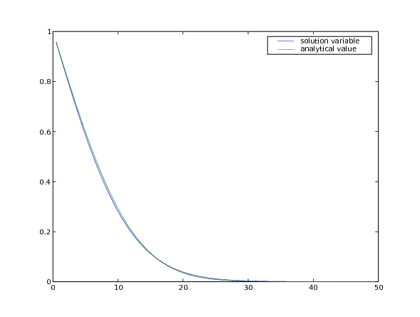
solution to diffusion problem evolved by implicit time steps

Note that although much larger stable timesteps can be taken with this implicit version (there is, in fact, no limit to how large an implicit timestep you can take for this particular problem), the solution is less accurate. One way to achieve a compromise between stability and accuracy is with the Crank-Nicholson scheme, represented by:

phi_new[j] = phi_old[j] + (D * dt / (2 * dx**2)) * \
                ((phi_new[j+1] - 2 * phi_new[j] + phi_new[j-1])
                 + (phi_old[j+1] - 2 * phi_old[j] + phi_old[j-1]))

which is essentially an average of the explicit and implicit schemes from above. This can be rendered in FiPy as easily as

>>> eqCN = eqX + eqI

We again reset the problem

>>> phi.setValue(valueRight)

and apply the Crank-Nicholson scheme until the end, when we apply one step of the fully implicit scheme to drive down the error (see, e.g., section 19.2 of [22]).

>>> from builtins import range
>>> for step in range(steps - 1):
...     eqCN.solve(var=phi,
...                dt=timeStepDuration)
...     if __name__ == '__main__':
...         viewer.plot()
>>> eqI.solve(var=phi,
...           dt=timeStepDuration)
>>> if __name__ == '__main__':
...     viewer.plot()

>>> print(phi.allclose(phiAnalytical, atol = 3e-3)) 
1

>>> from fipy import input
>>> if __name__ == '__main__':
...     input("Crank-Nicholson transient diffusion. Press <return> to proceed...")

As mentioned above, there is no stable limit to how large a time step can be taken for the implicit diffusion problem. In fact, if the time evolution of the problem is not interesting, it is possible to eliminate the time step altogether by omitting the TransientTerm. The steady-state diffusion equation

$D \nabla^2 \phi = 0$

is represented in FiPy by

>>> DiffusionTerm(coeff=D).solve(var=phi)

>>> if __name__ == '__main__':
...     viewer.plot()

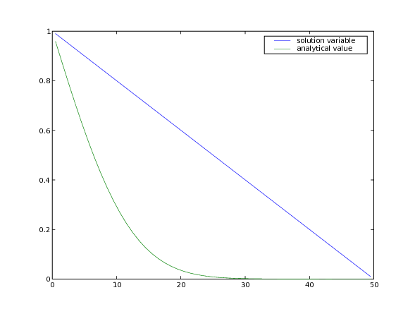
The analytical solution to the steady-state problem is no longer an error function, but simply a straight line, which we can confirm to a tolerance of $10^{-10}$ .

>>> L = nx * dx
>>> print(phi.allclose(valueLeft + (valueRight - valueLeft) * x / L,
...                    rtol = 1e-10, atol = 1e-10))
1

>>> from fipy import input
>>> if __name__ == '__main__':
...     input("Implicit steady-state diffusion. Press <return> to proceed...")

steady-state solution to diffusion problem

Often, boundary conditions may be functions of another variable in the system or of time.

For example, to have

$\phi = \begin{cases} (1 + \sin t) / 2 &\text{on $ x = 0 $} \\ 0 &\text{on $ x = L $} \\ \end{cases}$

we will need to declare time $t$ as a Variable

>>> time = Variable()

and then declare our boundary condition as a function of this Variable

>>> del phi.faceConstraints
>>> valueLeft = 0.5 * (1 + numerix.sin(time))
>>> phi.constrain(valueLeft, mesh.facesLeft)
>>> phi.constrain(0., mesh.facesRight)

>>> eqI = TransientTerm() == DiffusionTerm(coeff=D)

When we update time at each timestep, the left-hand boundary condition will automatically update,

>>> dt = .1
>>> while time() < 15:
...     time.setValue(time() + dt)
...     eqI.solve(var=phi, dt=dt)
...     if __name__ == '__main__':
...         viewer.plot()

>>> from fipy import input
>>> if __name__ == '__main__':
...     input("Time-dependent boundary condition. Press <return> to proceed...")

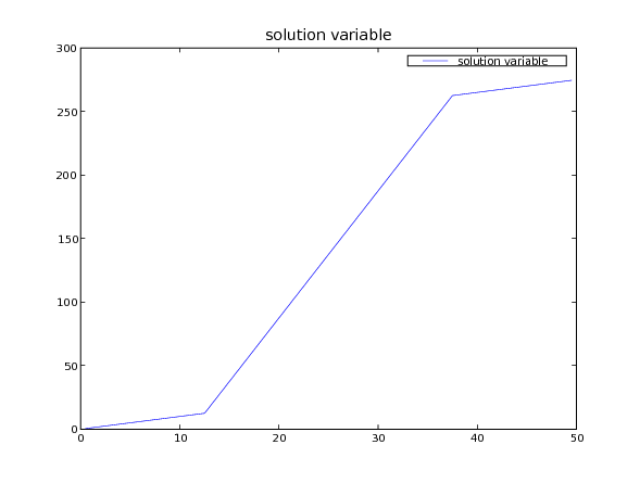
solution to diffusion problem with a time-dependent Dirichlet boundary condition

Many interesting problems do not have simple, uniform diffusivities. We consider a steady-state diffusion problem

$\nabla \cdot ( D \nabla \phi) = 0,$

with a spatially varying diffusion coefficient

$D = \begin{cases} 1& \text{for $ 0 < x < L / 4 $,} \\ 0.1& \text{for $ L / 4 \le x < 3 L / 4 $,} \\ 1& \text{for $ 3 L / 4 \le x < L $,} \end{cases}$

and with boundary conditions $\phi = 0$ at $x = 0$ and $D \frac{\partial \phi}{\partial x} = 1$ at $x = L$ , where $L$ is the length of the solution domain. Exact numerical answers to this problem are found when the mesh has cell centers that lie at $L / 4$ and $3 L / 4$ , or when the number of cells in the mesh $N_i$ satisfies $N_i = 4 i + 2$ , where $i$ is an integer. The mesh we’ve been using thus far is satisfactory, with $N_i = 50$ and $i = 12$ .

Because FiPy considers diffusion to be a flux from one cell to the next, through the intervening face, we must define the non-uniform diffusion coefficient on the mesh faces

>>> D = FaceVariable(mesh=mesh, value=1.0)
>>> X = mesh.faceCenters[0]
>>> D.setValue(0.1, where=(L / 4. <= X) & (X < 3. * L / 4.))

The boundary conditions are a fixed value of

>>> valueLeft = 0.

to the left and a fixed flux of

>>> fluxRight = 1.

to the right:

>>> phi = CellVariable(mesh=mesh)
>>> phi.faceGrad.constrain([fluxRight], mesh.facesRight)
>>> phi.constrain(valueLeft, mesh.facesLeft)

We re-initialize the solution variable

>>> phi.setValue(0)

and obtain the steady-state solution with one implicit solution step

>>> DiffusionTerm(coeff = D).solve(var=phi)

The analytical solution is simply

$\phi = \begin{cases} x & \text{for $ 0 < x < L/4 $,} \\ 10 x - 9L/4 & \text{for $ L/4 \le x < 3 L / 4 $,} \\ x + 18 L / 4 & \text{for $ 3 L / 4 \le x < L $,} \end{cases}$

or

>>> x = mesh.cellCenters[0]
>>> phiAnalytical.setValue(x)
>>> phiAnalytical.setValue(10 * x - 9. * L / 4.,
...                        where=(L / 4. <= x) & (x < 3. * L / 4.))
>>> phiAnalytical.setValue(x + 18. * L / 4.,
...                        where=3. * L / 4. <= x)
>>> print(phi.allclose(phiAnalytical, atol = 1e-8, rtol = 1e-8))
1

And finally, we can plot the result

>>> from fipy import input
>>> if __name__ == '__main__':
...     Viewer(vars=(phi, phiAnalytical)).plot()
...     input("Non-uniform steady-state diffusion. Press <return> to proceed...")

steady-state solution to diffusion problem with a non-uniform diffusivity

Note that for problems involving heat transfer and other similar conservation equations, it is important to ensure that we begin with the correct form of the equation. For example, for heat transfer with $\phi$ representing the temperature,

$\frac{\partial}{\partial t} \left(\rho \hat{C}_p \phi\right) = \nabla \cdot [ k \nabla \phi ].$

With constant and uniform density $\rho$ , heat capacity $\hat{C}_p$ and thermal conductivity $k$ , this is often written like Eq. (1), but replacing $D$ with $\alpha = \frac{k}{\rho \hat{C}_p}$ . However, when these parameters vary either in position or time, it is important to be careful with the form of the equation used. For example, if $k = 1$ and

$\rho \hat{C}_p = \begin{cases} 1& \text{for $ 0 < x < L / 4 $,} \\ 10& \text{for $ L / 4 \le x < 3 L / 4 $,} \\ 1& \text{for $ 3 L / 4 \le x < L $,} \end{cases},$

then we have

$\alpha = \begin{cases} 1& \text{for $ 0 < x < L / 4 $,} \\ 0.1& \text{for $ L / 4 \le x < 3 L / 4 $,} \\ 1& \text{for $ 3 L / 4 \le x < L $,} \end{cases}.$

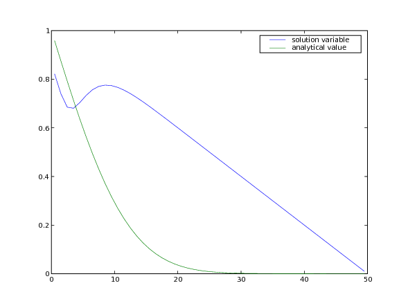
However, using a DiffusionTerm with the same coefficient as that in the section above is incorrect, as the steady state governing equation reduces to $0 = \nabla^2\phi$ , which results in a linear profile in 1D, unlike that for the case above with spatially varying diffusivity. Similar care must be taken if there is time dependence in the parameters in transient problems.

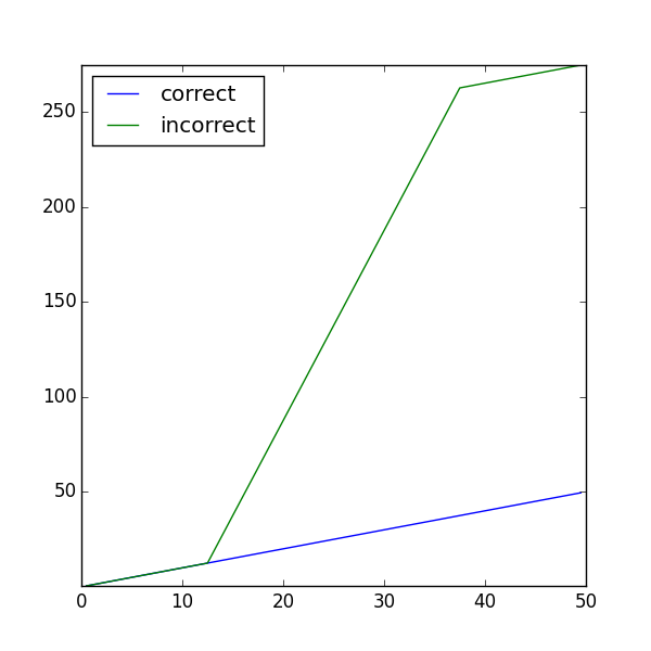
We can illustrate the differences with an example. We define field variables for the correct and incorrect solution

>>> phiT = CellVariable(name="correct", mesh=mesh)
>>> phiF = CellVariable(name="incorrect", mesh=mesh)
>>> phiT.faceGrad.constrain([fluxRight], mesh.facesRight)
>>> phiF.faceGrad.constrain([fluxRight], mesh.facesRight)
>>> phiT.constrain(valueLeft, mesh.facesLeft)
>>> phiF.constrain(valueLeft, mesh.facesLeft)
>>> phiT.setValue(0)
>>> phiF.setValue(0)

The relevant parameters are

>>> k = 1.
>>> alpha_false = FaceVariable(mesh=mesh, value=1.0)
>>> X = mesh.faceCenters[0]
>>> alpha_false.setValue(0.1, where=(L / 4. <= X) & (X < 3. * L / 4.))
>>> eqF = 0 == DiffusionTerm(coeff=alpha_false)
>>> eqT = 0 == DiffusionTerm(coeff=k)
>>> eqF.solve(var=phiF)
>>> eqT.solve(var=phiT)

Comparing to the correct analytical solution, $\phi = x$

>>> x = mesh.cellCenters[0]
>>> phiAnalytical.setValue(x)
>>> print(phiT.allclose(phiAnalytical, atol = 1e-8, rtol = 1e-8)) 
1

and finally, plot

>>> from fipy import input
>>> if __name__ == '__main__':
...     Viewer(vars=(phiT, phiF)).plot()
...     input("Non-uniform thermal conductivity. Press <return> to proceed...")

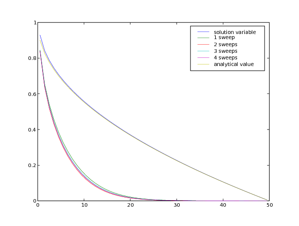
representation of difference between non-uniform alpha and D

Often, the diffusivity is not only non-uniform, but also depends on the value of the variable, such that

(2)¶ $\frac{\partial \phi}{\partial t} = \nabla \cdot [ D(\phi) \nabla \phi].$

With such a non-linearity, it is generally necessary to “sweep” the solution to convergence. This means that each time step should be calculated over and over, using the result of the previous sweep to update the coefficients of the equation, without advancing in time. In FiPy, this is accomplished by creating a solution variable that explicitly retains its “old” value by specifying hasOld when you create it. The variable does not move forward in time until it is explicitly told to updateOld(). In order to compare the effects of different numbers of sweeps, let us create a list of variables: phi[0] will be the variable that is actually being solved and phi[1] through phi[4] will display the result of taking the corresponding number of sweeps (phi[1] being equivalent to not sweeping at all).

>>> valueLeft = 1.
>>> valueRight = 0.
>>> phi = [
...     CellVariable(name="solution variable",
...                  mesh=mesh,
...                  value=valueRight,
...                  hasOld=1),
...     CellVariable(name="1 sweep",
...                  mesh=mesh),
...     CellVariable(name="2 sweeps",
...                  mesh=mesh),
...     CellVariable(name="3 sweeps",
...                  mesh=mesh),
...     CellVariable(name="4 sweeps",
...                  mesh=mesh)
... ]

If, for example,

$D = D_0 (1 - \phi)$

we would simply write Eq. (2) as

>>> D0 = 1.
>>> eq = TransientTerm() == DiffusionTerm(coeff=D0 * (1 - phi[0]))

Note

Because of the non-linearity, the Crank-Nicholson scheme does not work for this problem.

We apply the same boundary conditions that we used for the uniform diffusivity cases

>>> phi[0].constrain(valueRight, mesh.facesRight)
>>> phi[0].constrain(valueLeft, mesh.facesLeft)

Although this problem does not have an exact transient solution, it can be solved in steady-state, with

$\phi(x) = 1 - \sqrt{\frac{x}{L}}$

>>> x = mesh.cellCenters[0]
>>> phiAnalytical.setValue(1. - numerix.sqrt(x/L))

We create a viewer to compare the different numbers of sweeps with the analytical solution from before.

>>> if __name__ == '__main__':
...     viewer = Viewer(vars=phi + [phiAnalytical],
...                     datamin=0., datamax=1.)
...     viewer.plot()

As described above, an inner “sweep” loop is generally required for the solution of non-linear or multiple equation sets. Often a conditional is required to exit this “sweep” loop given some convergence criteria. Instead of using the solve() method equation, when sweeping, it is often useful to call sweep() instead. The sweep() method behaves the same way as solve(), but returns the residual that can then be used as part of the exit condition.

We now repeatedly run the problem with increasing numbers of sweeps.

>>> from fipy import input
>>> from builtins import range
>>> for sweeps in range(1, 5):
...     phi[0].setValue(valueRight)
...     for step in range(steps):
...         # only move forward in time once per time step
...         phi[0].updateOld()
...
...         # but "sweep" many times per time step
...         for sweep in range(sweeps):
...             res = eq.sweep(var=phi[0],
...                            dt=timeStepDuration)
...         if __name__ == '__main__':
...             viewer.plot()
...
...     # copy the final result into the appropriate display variable
...     phi[sweeps].setValue(phi[0])
...     if __name__ == '__main__':
...         viewer.plot()
...         input("Implicit variable diffusivity. %d sweep(s). \
... Residual = %f. Press <return> to proceed..." % (sweeps, (abs(res))))

As can be seen, sweeping does not dramatically change the result, but the “residual” of the equation (a measure of how accurately it has been solved) drops about an order of magnitude with each additional sweep.

Attention

Choosing an optimal balance between the number of time steps, the number of sweeps, the number of solver iterations, and the solver tolerance is more art than science and will require some experimentation on your part for each new problem.

Finally, we can increase the number of steps to approach equilibrium, or we can just solve for it directly

>>> eq = DiffusionTerm(coeff=D0 * (1 - phi[0]))

>>> phi[0].setValue(valueRight)
>>> res = 1e+10
>>> while res > 1e-6:
...     res = eq.sweep(var=phi[0],
...                    dt=timeStepDuration)

>>> print(phi[0].allclose(phiAnalytical, atol = 1e-1))
1

>>> from fipy import input
>>> if __name__ == '__main__':
...     viewer.plot()
...     input("Implicit variable diffusivity - steady-state. \
... Press <return> to proceed...")

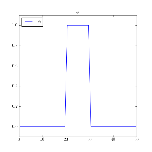
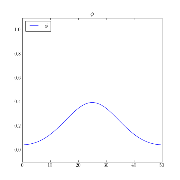
solution to a diffusion problem a non-linear diffusivity

Fully implicit solutions are not without their pitfalls, particularly in steady state. Consider a localized block of material diffusing in a closed box.

>>> phi = CellVariable(mesh=mesh, name=r"$\phi$")

>>> phi.value = 0.
>>> phi.setValue(1., where=(x > L/2. - L/10.) & (x < L/2. + L/10.))
>>> if __name__ == '__main__':
...     viewer = Viewer(vars=phi, datamin=-0.1, datamax=1.1)

initial condition for no-flux boundary conditions

We assign no explicit boundary conditions, leaving the default no-flux boundary conditions, and solve

$\partial\phi/\partial t = \nabla\cdot(D\nabla\phi)$

>>> D = 1.
>>> eq = TransientTerm() == DiffusionTerm(D)

>>> dt = 10. * dx**2 / (2 * D)
>>> steps = 200

>>> from builtins import range
>>> for step in range(steps):
...     eq.solve(var=phi, dt=dt)
...     if __name__ == '__main__':
...         viewer.plot()
>>> from fipy import input
>>> if __name__ == '__main__':
...     input("No-flux - transient. \
... Press <return> to proceed...")

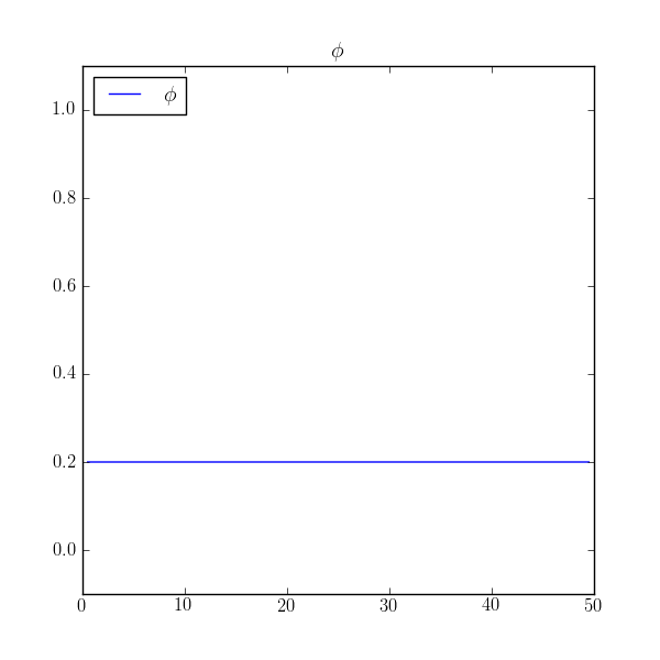
long-time solution for no-flux boundary conditions

and see that $\phi$ dissipates to the expected average value of 0.2 with reasonable accuracy.

>>> print(numerix.allclose(phi, 0.2, atol=1e-5))
True

If we reset the initial condition

>>> phi.value = 0.
>>> phi.setValue(1., where=(x > L/2. - L/10.) & (x < L/2. + L/10.))
>>> if __name__ == '__main__':
...     viewer.plot()

and solve the steady-state problem

>>> DiffusionTerm(coeff=D).solve(var=phi) 
>>> if __name__ == '__main__':
...     viewer.plot()
>>> from fipy import input
>>> if __name__ == '__main__':
...     input("No-flux - stead-state failure. \
... Press <return> to proceed...")

>>> print(numerix.allclose(phi, 0.0)) 
True

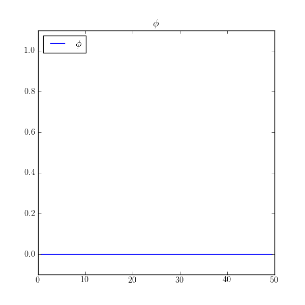
(failed) steady-state solution for no-flux boundary conditions

we find that the value is uniformly zero! What happened to our no-flux boundary conditions?

The problem is that in the implicit discretization of $\nabla\cdot(D\nabla\phi) = 0$ ,

$\begin{vmatrix} \frac{D}{{\Delta x}^2} & -\frac{D}{{\Delta x}^2} & & & & & \\\\[1em] \ddots & \ddots & \ddots & & & & \\[1em] & -\frac{D}{{\Delta x}^2} & \frac{2 D}{{\Delta x}^2} & -\frac{D}{{\Delta x}^2} & & & \\\\[1em] & & -\frac{D}{{\Delta x}^2} & \frac{2 D}{{\Delta x}^2} & -\frac{D}{{\Delta x}^2} & & \\\\[1em] & & & -\frac{D}{{\Delta x}^2} & \frac{2 D}{{\Delta x}^2} & -\frac{D}{{\Delta x}^2} & \\\\[1em] & & & & \ddots & \ddots & \ddots \\\\[1em] & & & & & -\frac{D}{{\Delta x}^2} & \frac{D}{{\Delta x}^2} \\\\[1em] \end{vmatrix} \begin{vmatrix} \phi^\text{new}_{0} \\\\[1em] \vdots \\[1em] \phi^\text{new}_{j-1} \\\\[1em] \phi^\text{new}_{j} \\\\[1em] \phi^\text{new}_{j+1} \\\\[1em] \vdots \\\\[1em] \phi^\text{new}_{N-1} \end{vmatrix} = \begin{vmatrix} 0 \\\\[1em] \vdots \\\\[1em] 0 \\\\[1em] 0 \\\\[1em] 0 \\\\[1em] \vdots \\\\[1em] 0 \end{vmatrix}$

the initial condition $\phi^\text{old}$ no longer appears and $\phi = 0$ is a perfectly legitimate solution to this matrix equation.

The solution is to run the transient problem and to take one enormous time step

>>> phi.value = 0.
>>> phi.setValue(1., where=(x > L/2. - L/10.) & (x < L/2. + L/10.))
>>> if __name__ == '__main__':
...     viewer.plot()

>>> (TransientTerm() == DiffusionTerm(D)).solve(var=phi, dt=1e6*dt)
>>> if __name__ == '__main__':
...     viewer.plot()
>>> from fipy import input
>>> if __name__ == '__main__':
...     input("No-flux - steady-state. \
... Press <return> to proceed...")

>>> print(numerix.allclose(phi, 0.2, atol=1e-5))
True

steady-state solution for no-flux boundary conditions

If this example had been written primarily as a script, instead of as documentation, we would delete every line that does not begin with either “>>>” or “...”, and then delete those prefixes from the remaining lines, leaving:

## This script was derived from
## 'examples/diffusion/mesh1D.py'

nx = 50
dx = 1.
mesh = Grid1D(nx = nx, dx = dx)
phi = CellVariable(name="solution variable",
                   mesh=mesh,
                   value=0)

eq = DiffusionTerm(coeff=D0 * (1 - phi[0]))
phi[0].setValue(valueRight)
res = 1e+10
while res > 1e-6:
    res = eq.sweep(var=phi[0],
                   dt=timeStepDuration)

print phi[0].allclose(phiAnalytical, atol = 1e-1)
# Expect:
# 1
#
if __name__ == '__main__':
    viewer.plot()
    input("Implicit variable diffusivity - steady-state. \
Press <return> to proceed...")

Your own scripts will tend to look like this, although you can always write them as doctest scripts if you choose. You can obtain a plain script like this from some …/example.py by typing:

$ python setup.py copy_script --From .../example.py --To myExample.py

at the command line.

Most of the FiPy examples will be a mixture of plain scripts and doctest documentation/tests.

Last updated on Jun 27, 2023. Created using Sphinx 6.2.1.