-
Citation: J. Byggmästar, M. Nagel, K. Albe, K. Henriksson, and K. Nordlund (2019), "Analytical interatomic bond-order potential for simulations of oxygen defects in iron", Journal of Physics: Condensed Matter 31, 215401. DOI: 10.1088/1361-648x/ab0931.Abstract: We present an analytical bond-order potential for the Fe–O system, capable of reproducing the basic properties of wüstite as well as the energetics of oxygen impurities in α-iron. The potential predicts binding energies of various small oxygen-vacancy clusters in α-iron in good agreement with density functional theory results, and is therefore suitable for simulations of oxygen-based defects in iron. We apply the potential in simulations of the stability and structure of Fe/FeO interfaces and FeO precipitates in iron, and observe that the shape of FeO precipitates can change due to formation of well-defined Fe/FeO interfaces. The interface with crystalline Fe also ensures that the precipitates never become fully amorphous, no matter how small they are.
Notes: The potential is not suitable for simulations of the Fe2O3 and Fe3O4 phases.
Related Models: -
LAMMPS pair_style tersoff/zbl (2019--Byggmastar-J--Fe-O--LAMMPS--ipr1)See Computed Properties
Notes: This file was provided by Jesper Byggmästar (University of Helsinki) on 20 March 2019 and posted with his permission.
File(s):
Implementation Information
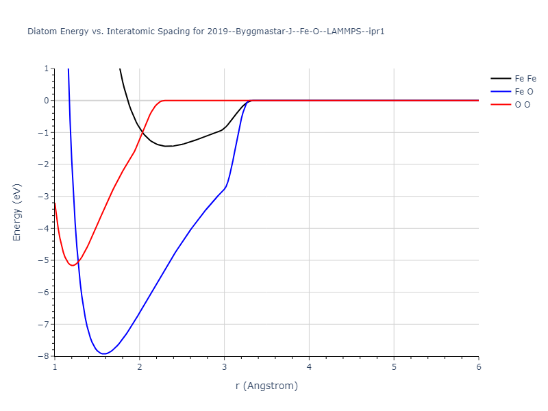
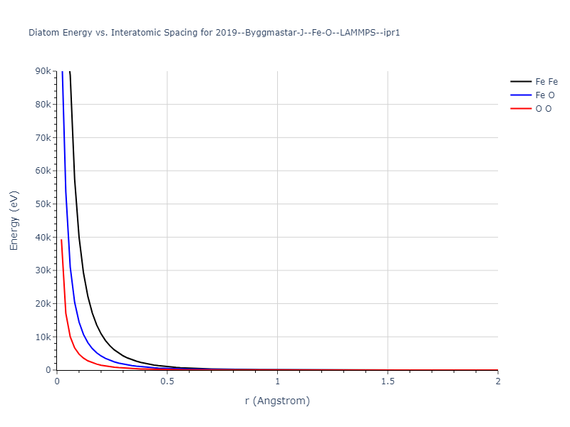
Diatom Energy vs. Interatomic Spacing
Plots of the potential energy vs interatomic spacing, r, are shown below for all diatom sets associated with the interatomic potential. This calculation provides insights into the functional form of the potential's two-body interactions. A system consisting of only two atoms is created, and the potential energy is evaluated for the atoms separated by 0.02 Å <= r <= 6.0> Å in intervals of 0.02 Å. Two plots are shown: one for the "standard" interaction distance range, and one for small values of r. The small r plot is useful for determining whether the potential is suitable for radiation studies.
The calculation method used is available as the iprPy diatom_scan calculation method.
Clicking on the image of a plot will open an interactive version of it in a new tab. The underlying data for the plots can be downloaded by clicking on the links above each plot.
Notes and Disclaimers:
- These values are meant to be guidelines for comparing potentials, not the absolute values for any potential's properties. Values listed here may change if the calculation methods are updated due to improvements/corrections. Variations in the values may occur for variations in calculation methods, simulation software and implementations of the interatomic potentials.
- As this calculation only involves two atoms, it neglects any multi-body interactions that may be important in molecules, liquids and crystals.
- NIST disclaimer
Version Information:
- 2019-11-14. Maximum value range on the shortrange plots are now limited to "expected" levels as details are otherwise lost.
- 2019-08-07. Plots added.
Click on plot to load interactive version
Click on plot to load interactive version
Cohesive Energy vs. Interatomic Spacing
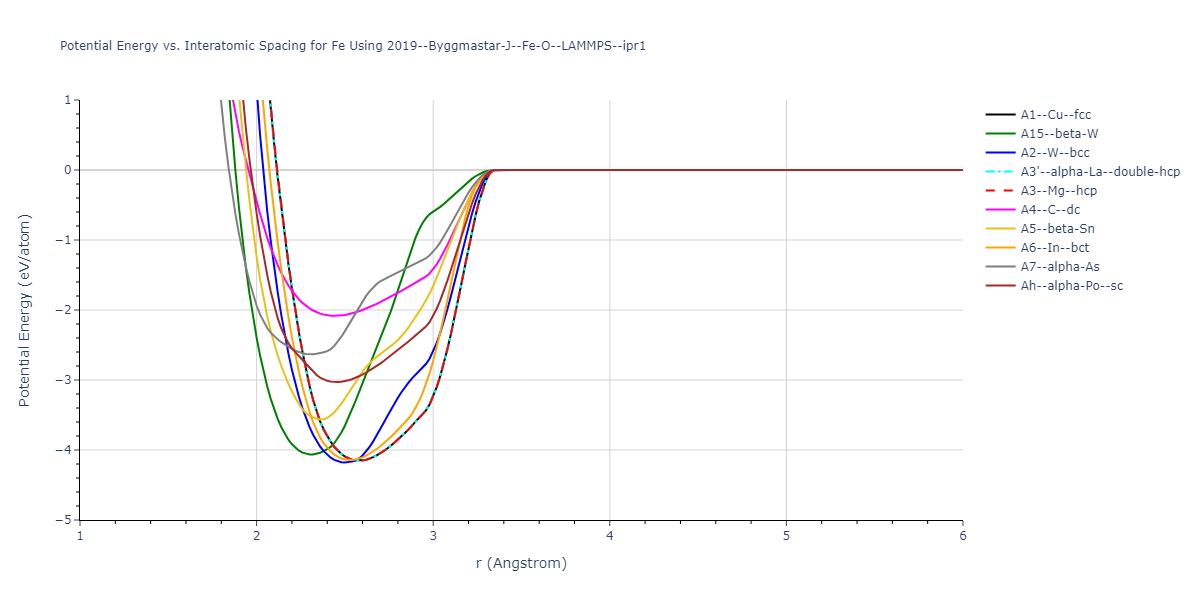
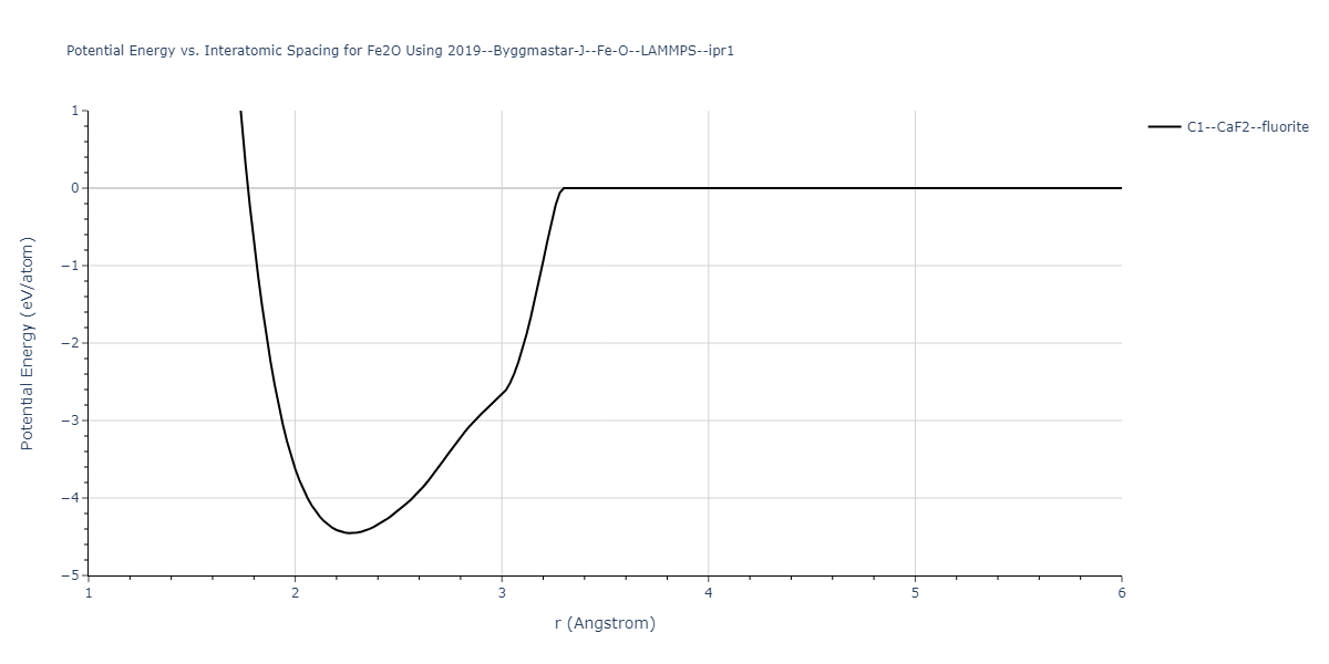
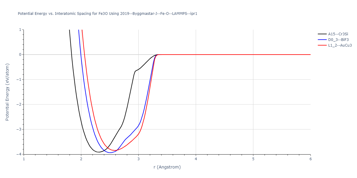
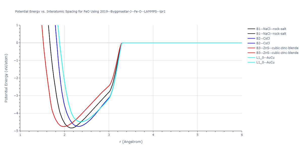
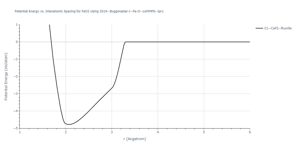
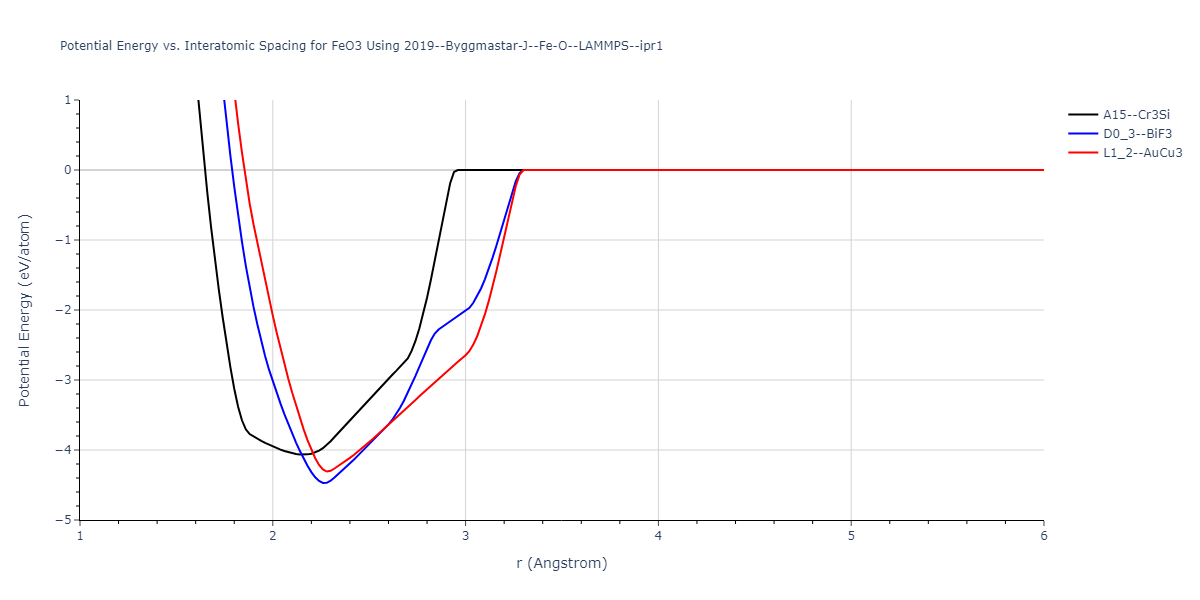
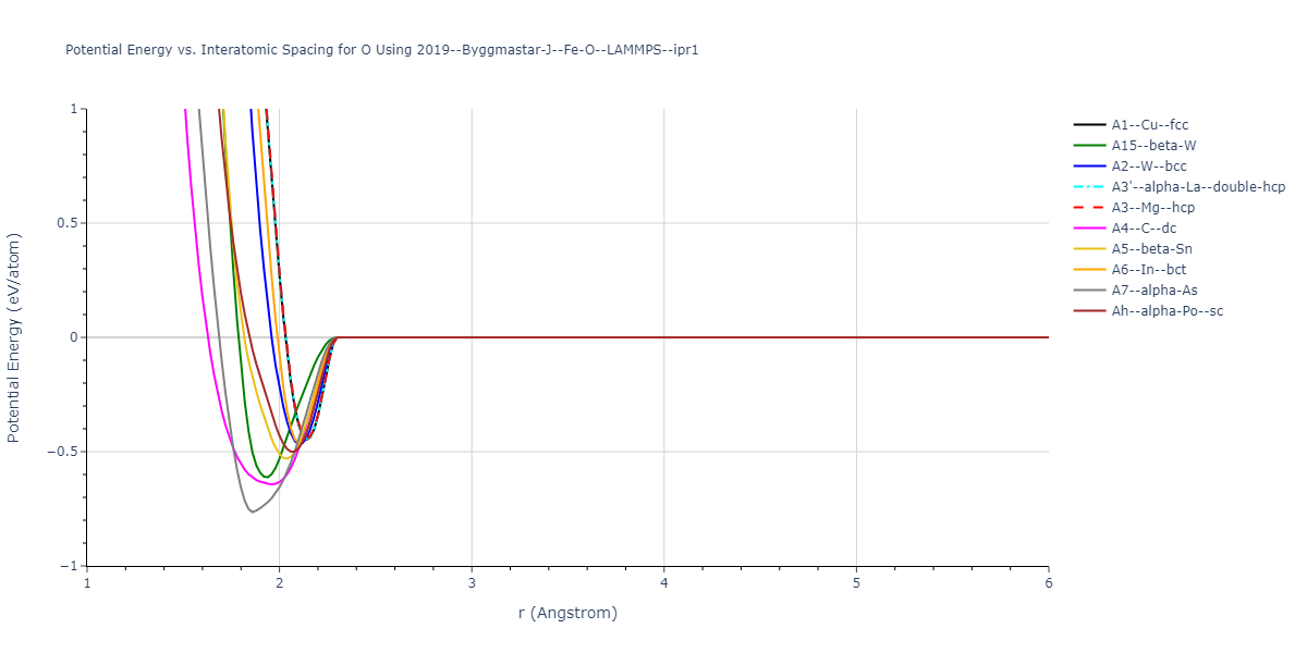
Plots of potential energy vs interatomic spacing, r, are shown below for a number of crystal structures. The structures are generated based on the ideal atomic positions and b/a and c/a lattice parameter ratios for a given crystal prototype. The size of the system is then uniformly scaled, and the energy calculated without relaxing the system. To obtain these plots, values of r are evaluated every 0.02 Å up to 6 Å.
The calculation method used is available as the iprPy E_vs_r_scan calculation method.
Clicking on the image of a plot will open an interactive version of it in a new tab. The underlying data for the plots can be downloaded by clicking on the links above each plot.
Notes and Disclaimers:
- These values are meant to be guidelines for comparing potentials, not the absolute values for any potential's properties. Values listed here may change if the calculation methods are updated due to improvements/corrections. Variations in the values may occur for variations in calculation methods, simulation software and implementations of the interatomic potentials.
- The minima identified by this calculation do not guarantee that the associated crystal structures will be stable since no relaxation is performed.
- NIST disclaimer
Version Information:
- 2020-12-18. Descriptions, tables and plots updated to reflect that the energy values are the measuredper atom potential energy rather than cohesive energy as some potentials have non-zero isolated atom energies.
- 2019-02-04. Values regenerated with even r spacings of 0.02 Å, and now include values less than 2 Å when possible. Updated calculation method and parameters enhance compatibility with more potential styles.
- 2019-04-26. Results for hcp, double hcp, α-As and L10 prototypes regenerated from different unit cell representations. Only α-As results show noticable (>1e-5 eV) difference due to using a different coordinate for Wykoff site c position.
- 2018-06-13. Values for MEAM potentials corrected. Dynamic versions of the plots moved to separate pages to improve page loading. Cosmetic changes to how data is shown and updates to the documentation.
- 2017-01-11. Replaced png pictures with interactive Bokeh plots. Data regenerated with 200 values of r instead of 300.
- 2016-09-28. Plots for binary structures added. Data and plots for elemental structures regenerated. Data values match the values of the previous version. Data table formatting slightly changed to increase precision and ensure spaces between large values. Composition added to plot title and structure names made longer.
- 2016-04-07. Plots for elemental structures added.
Crystal Structure Predictions
Computed lattice constants and cohesive/potential energies are displayed for a variety of crystal structures. The values displayed here are obtained using the following process.
- Initial crystal structure guesses are taken from:
- The iprPy E_vs_r_scan calculation results (shown above) by identifying all energy minima along the measured curves for a given crystal prototype + composition.
- Structures in the Materials Project and OQMD DFT databases.
- All initial guesses are relaxed using three independent methods using a 10x10x10 supercell:
- "box": The system's lattice constants are adjusted to zero pressure without internal relaxations using the iprPy relax_box calculation with a strainrange of 1e-6.
- "static": The system's lattice and atomic positions are statically relaxed using the iprPy relax_static calculation with a minimization force tolerance of 1e-10 eV/Angstrom.
- "dynamic": The system's lattice and atomic positions are dynamically relaxed for 10000 timesteps of 0.01 ps using the iprPy relax_dynamic calculation with an nph integration plus Langevin thermostat. The final configuration is then used as input in running an iprPy relax_static calculation with a minimization force tolerance of 1e-10 eV/Angstrom.
- The relaxed structures obtained from #2 are then evaluated using the spglib package to identify an ideal crystal unit cell based on the results.
- The space group information of the ideal unit cells is compared to the space group information of the corresponding reference structures to identify which structures transformed upon relaxation. The structures that did not transform to a different structure are listed in the table(s) below. The "method" field indicates the most rigorous relaxation method where the structure did not transform. The space group information is also used to match the DFT reference structures to the used prototype, where possible.
- The cohesive energy, Ecoh, is calculated from the measured potential energy per atom, Epot$, by subtracting the isolated energy averaged across all atoms in the unit cell. The isolated atom energies of each species model is obtained either by evaluating a single atom atomic configuration, or by identifying the first energy plateau from the diatom scan calculations for r > 2 Å.
The calculation methods used are implemented into iprPy as the following calculation styles
Notes and Disclaimers:
- These values are meant to be guidelines for comparing potentials, not the absolute values for any potential's properties. Values listed here may change if the calculation methods are updated due to improvements/corrections. Variations in the values may occur for variations in calculation methods, simulation software and implementations of the interatomic potentials.
- The presence of any structures in this list does not guarantee that those structures are stable. Also, the lowest energy structure may not be included in this list.
- Multiple values for the same crystal structure but different lattice constants are possible. This is because multiple energy minima are possible for a given structure and interatomic potential. Having multiple energy minima for a structure does not necessarily make the potential "bad" as unwanted configurations may be unstable or correspond to conditions that may not be relevant to the problem of interest (eg. very high strains).
- NIST disclaimer
Version Information:
- 2025-07-02. All "mp-" reference structure calculations were re-relaxed using the updated Materials Project database rather than the original database structures. Also, a bug was fixed that caused the "static" relaxations to occasionally throw unnecessary errors. This was fixed and all affected calculations were reset and performed again.
- 2022-05-27. The "box" method results have all been redone with an updated methodology more suited for non-orthogonal systems.
- 2020-12-18. Cohesive energies have been corrected by making them relative to the energies of the isolated atoms. The previous cohesive energy values are now listed as the potential energies.
- 2019-06-07. Structures with positive or near zero cohesive energies removed from the display tables. All values still present in the raw data files.
- 2019-04-26. Calculations now computed for each implementation. Results for hcp, double hcp, α-As and L10 prototypes regenerated from different unit cell representations.
- 2018-06-14. Methodology completely changed affecting how the information is displayed. Calculations involving MEAM potentials corrected.
- 2016-09-28. Values for simple compounds added. All identified energy minima for each structure are listed. The existing elemental data was regenerated. Most values are consistent with before, but some differences have been noted. Specifically, variations are seen with some values for potentials where the elastic constants don't vary smoothly near the equilibrium state. Additionally, the inclusion of some high-energy structures has changed based on new criteria for identifying when structures have relaxed to another structure.
- 2016-04-07. Values for elemental crystal structures added. Only values for the global energy minimum of each unique structure given.
Download raw data (including filtered results)
Reference structure matches:
A1--Cu--fcc = mp-150, oqmd-7505, oqmd-1214525
A15--beta-W = oqmd-1214970
A2--W--bcc = mp-13, oqmd-8568, oqmd-22514, oqmd-1215148
A3'--alpha-La--double-hcp = oqmd-1215416
A3--Mg--hcp = mp-136, oqmd-30158, oqmd-51781, oqmd-1215326, oqmd-1215391
A4--C--dc = oqmd-1215505
A5--beta-Sn = oqmd-1215594
A6--In--bct = oqmd-1215683
Ah--alpha-Po--sc = mp-568345
| prototype | method | Ecoh (eV/atom) | Epot (eV/atom) | a0 (Å) | b0 (Å) | c0 (Å) | α (degrees) | β (degrees) | γ (degrees) |
|---|---|---|---|---|---|---|---|---|---|
| A2--W--bcc | dynamic | -4.1787 | -4.1787 | 2.8886 | 2.8886 | 2.8886 | 90.0 | 90.0 | 90.0 |
| A3--Mg--hcp | dynamic | -4.1545 | -4.1545 | 2.5809 | 2.5809 | 4.2042 | 90.0 | 90.0 | 120.0 |
| oqmd-1216039 | dynamic | -4.1534 | -4.1534 | 2.5803 | 2.5803 | 18.9299 | 90.0 | 90.0 | 120.0 |
| oqmd-1216039 | box | -4.1533 | -4.1533 | 2.5803 | 2.5803 | 18.9301 | 90.0 | 90.0 | 120.0 |
| A3'--alpha-La--double-hcp | dynamic | -4.1528 | -4.1528 | 2.58 | 2.58 | 8.4158 | 90.0 | 90.0 | 120.0 |
| A1--Cu--fcc | dynamic | -4.1511 | -4.1511 | 3.6473 | 3.6473 | 3.6473 | 90.0 | 90.0 | 90.0 |
| oqmd-1215237 | box | -4.1262 | -4.1262 | 2.528 | 4.5362 | 4.2415 | 90.0 | 90.0 | 90.0 |
| oqmd-1214792 | dynamic | -4.0802 | -4.0802 | 8.9154 | 8.9154 | 8.9154 | 90.0 | 90.0 | 90.0 |
| oqmd-1214792 | box | -4.0767 | -4.0767 | 8.9159 | 8.9159 | 8.9159 | 90.0 | 90.0 | 90.0 |
| A15--beta-W | dynamic | -4.0643 | -4.0643 | 4.6172 | 4.6172 | 4.6172 | 90.0 | 90.0 | 90.0 |
| oqmd-1214881 | box | -4.0477 | -4.0477 | 6.2644 | 6.2644 | 6.2644 | 90.0 | 90.0 | 90.0 |
| oqmd-21053 | dynamic | -3.9986 | -3.9986 | 8.7238 | 8.7238 | 4.675 | 90.0 | 90.0 | 90.0 |
| mp-1194030 | static | -3.9827 | -3.9827 | 8.6472 | 8.6472 | 4.6927 | 90.0 | 90.0 | 90.0 |
| oqmd-21053 | static | -3.982 | -3.982 | 8.6448 | 8.6448 | 4.6899 | 90.0 | 90.0 | 90.0 |
| mp-1245108 | dynamic | -3.9754 | -3.9754 | 10.6054 | 10.7584 | 10.9626 | 87.6 | 89.7 | 88.8 |
| oqmd-21053 | box | -3.9709 | -3.9709 | 8.6288 | 8.6288 | 4.6844 | 90.0 | 90.0 | 90.0 |
| mp-1194030 | box | -3.9517 | -3.9517 | 8.5844 | 8.5844 | 4.7009 | 90.0 | 90.0 | 90.0 |
| mp-1245108 | static | -3.9332 | -3.9332 | 10.6069 | 10.6722 | 10.9536 | 92.0 | 90.4 | 91.4 |
| mp-1245108 | box | -3.9306 | -3.9306 | 10.6075 | 10.6707 | 10.9513 | 92.0 | 90.5 | 91.4 |
| oqmd-1215059 | box | -3.8479 | -3.8479 | 2.6541 | 4.1605 | 9.0613 | 90.0 | 90.0 | 90.0 |
| A5--beta-Sn | dynamic | -3.5806 | -3.5806 | 4.6447 | 4.6447 | 2.4395 | 90.0 | 90.0 | 90.0 |
| mp-1096950 | box | -3.4823 | -3.4823 | 2.509 | 2.509 | 2.4824 | 90.0 | 90.0 | 120.0 |
| Ah--alpha-Po--sc | static | -3.0302 | -3.0302 | 2.4529 | 2.4529 | 2.4529 | 90.0 | 90.0 | 90.0 |
| oqmd-21731 | box | -3.0301 | -3.0301 | 2.4529 | 2.4529 | 7.3587 | 90.0 | 90.0 | 90.0 |
| oqmd-1215950 | box | -2.8105 | -2.8105 | 3.8616 | 4.0498 | 3.8694 | 90.0 | 119.8 | 90.0 |
| A4--C--dc | box | -2.0839 | -2.0839 | 5.6409 | 5.6409 | 5.6409 | 90.0 | 90.0 | 90.0 |
Download raw data (including filtered results)
Reference structure matches:
| prototype | method | Ecoh (eV/atom) | Epot (eV/atom) | a0 (Å) | b0 (Å) | c0 (Å) | α (degrees) | β (degrees) | γ (degrees) |
|---|---|---|---|---|---|---|---|---|---|
| mp-705555 | dynamic | -4.7955 | -4.7955 | 6.7995 | 6.8002 | 10.5883 | 105.0 | 97.7 | 107.3 |
| mp-759504 | dynamic | -4.7953 | -4.7953 | 5.2839 | 6.8038 | 6.8051 | 107.4 | 105.0 | 97.6 |
| mp-759504 | static | -4.7953 | -4.7953 | 5.2838 | 6.8039 | 6.8051 | 107.4 | 105.0 | 97.6 |
| mp-705555 | box | -4.7765 | -4.7765 | 6.782 | 6.7913 | 10.5831 | 104.9 | 97.7 | 107.4 |
| mp-759504 | box | -4.7754 | -4.7754 | 5.2777 | 6.7898 | 6.7956 | 107.4 | 98.1 | 105.0 |
Download raw data (including filtered results)
Reference structure matches:
| prototype | method | Ecoh (eV/atom) | Epot (eV/atom) | a0 (Å) | b0 (Å) | c0 (Å) | α (degrees) | β (degrees) | γ (degrees) |
|---|---|---|---|---|---|---|---|---|---|
| mp-705417 | dynamic | -4.7993 | -4.7993 | 6.1112 | 6.7979 | 6.803 | 95.6 | 102.8 | 116.7 |
| mp-705417 | static | -4.7993 | -4.7993 | 6.1112 | 6.7979 | 6.803 | 95.6 | 102.8 | 116.7 |
| mp-705417 | box | -4.7819 | -4.7819 | 6.1077 | 6.7605 | 6.7998 | 72.8 | 77.2 | 63.3 |
Download raw data (including filtered results)
Reference structure matches:
| prototype | method | Ecoh (eV/atom) | Epot (eV/atom) | a0 (Å) | b0 (Å) | c0 (Å) | α (degrees) | β (degrees) | γ (degrees) |
|---|---|---|---|---|---|---|---|---|---|
| mp-764326 | dynamic | -4.8026 | -4.8026 | 10.9649 | 10.9649 | 7.4874 | 90.0 | 90.0 | 120.0 |
| mp-764326 | static | -4.8026 | -4.8026 | 10.965 | 10.965 | 7.4872 | 90.0 | 90.0 | 120.0 |
| mp-764326 | box | -4.7926 | -4.7926 | 10.9359 | 10.9359 | 7.4794 | 90.0 | 90.0 | 120.0 |
Download raw data (including filtered results)
Reference structure matches:
| prototype | method | Ecoh (eV/atom) | Epot (eV/atom) | a0 (Å) | b0 (Å) | c0 (Å) | α (degrees) | β (degrees) | γ (degrees) |
|---|---|---|---|---|---|---|---|---|---|
| mp-705414 | dynamic | -4.8053 | -4.8053 | 8.0708 | 8.0708 | 14.8855 | 90.0 | 90.0 | 120.0 |
| mp-705414 | static | -4.8052 | -4.8052 | 8.0705 | 8.0705 | 14.8863 | 90.0 | 90.0 | 120.0 |
| mp-705414 | box | -4.7843 | -4.7843 | 8.0583 | 8.0583 | 14.7987 | 90.0 | 90.0 | 120.0 |
Download raw data (including filtered results)
Reference structure matches:
| prototype | method | Ecoh (eV/atom) | Epot (eV/atom) | a0 (Å) | b0 (Å) | c0 (Å) | α (degrees) | β (degrees) | γ (degrees) |
|---|---|---|---|---|---|---|---|---|---|
| mp-756693 | static | -4.7627 | -4.7627 | 5.2821 | 6.7959 | 9.0814 | 72.7 | 73.3 | 82.3 |
| mp-756693 | box | -4.7422 | -4.7422 | 5.2668 | 6.8382 | 9.0504 | 102.7 | 106.7 | 98.0 |
Download raw data (including filtered results)
Reference structure matches:
| prototype | method | Ecoh (eV/atom) | Epot (eV/atom) | a0 (Å) | b0 (Å) | c0 (Å) | α (degrees) | β (degrees) | γ (degrees) |
|---|---|---|---|---|---|---|---|---|---|
| mp-1195927 | box | -4.7359 | -4.7359 | 21.9088 | 3.0118 | 10.5984 | 90.0 | 118.6 | 90.0 |
| mp-1195927 | static | -4.7355 | -4.7355 | 21.966 | 2.9882 | 10.6355 | 90.0 | 118.5 | 90.0 |
Download raw data (including filtered results)
Reference structure matches:
| prototype | method | Ecoh (eV/atom) | Epot (eV/atom) | a0 (Å) | b0 (Å) | c0 (Å) | α (degrees) | β (degrees) | γ (degrees) |
|---|---|---|---|---|---|---|---|---|---|
| mp-764417 | dynamic | -4.8071 | -4.8071 | 6.8139 | 6.8139 | 12.9144 | 90.0 | 90.0 | 90.0 |
| mp-764417 | box | -4.7992 | -4.7992 | 6.8075 | 6.8075 | 12.9231 | 90.0 | 90.0 | 90.0 |
Download raw data (including filtered results)
Reference structure matches:
| prototype | method | Ecoh (eV/atom) | Epot (eV/atom) | a0 (Å) | b0 (Å) | c0 (Å) | α (degrees) | β (degrees) | γ (degrees) |
|---|---|---|---|---|---|---|---|---|---|
| mp-1224936 | dynamic | -4.7565 | -4.7565 | 6.0389 | 6.0389 | 31.0996 | 90.0 | 90.0 | 120.0 |
| mp-1224936 | box | -4.7345 | -4.7345 | 6.0086 | 6.0086 | 31.3652 | 90.0 | 90.0 | 120.0 |
| mp-705551 | static | -4.7332 | -4.7332 | 6.1573 | 6.1762 | 8.6012 | 91.1 | 91.3 | 90.2 |
| mp-705551 | box | -4.731 | -4.731 | 6.1578 | 6.1782 | 8.6018 | 91.1 | 91.3 | 90.2 |
Download raw data (including filtered results)
Reference structure matches:
| prototype | method | Ecoh (eV/atom) | Epot (eV/atom) | a0 (Å) | b0 (Å) | c0 (Å) | α (degrees) | β (degrees) | γ (degrees) |
|---|---|---|---|---|---|---|---|---|---|
| mp-705424 | dynamic | -4.812 | -4.812 | 6.8116 | 8.0579 | 8.0614 | 64.6 | 85.1 | 65.1 |
| mp-705424 | box | -4.7894 | -4.7894 | 6.8008 | 8.0519 | 8.0663 | 64.8 | 85.3 | 65.1 |
Download raw data (including filtered results)
Reference structure matches:
| prototype | method | Ecoh (eV/atom) | Epot (eV/atom) | a0 (Å) | b0 (Å) | c0 (Å) | α (degrees) | β (degrees) | γ (degrees) |
|---|---|---|---|---|---|---|---|---|---|
| mp-706875 | box | -4.7778 | -4.7778 | 6.7953 | 8.0414 | 9.6164 | 83.2 | 73.9 | 65.1 |
Download raw data (including filtered results)
Reference structure matches:
| prototype | method | Ecoh (eV/atom) | Epot (eV/atom) | a0 (Å) | b0 (Å) | c0 (Å) | α (degrees) | β (degrees) | γ (degrees) |
|---|---|---|---|---|---|---|---|---|---|
| mp-530048 | dynamic | -4.6865 | -4.6865 | 10.9403 | 10.9403 | 15.7771 | 90.0 | 90.0 | 120.0 |
| mp-530048 | static | -4.5994 | -4.5994 | 11.7334 | 11.7334 | 14.9951 | 90.0 | 90.0 | 120.0 |
| mp-530048 | box | -4.5512 | -4.5512 | 11.9731 | 11.9731 | 15.0832 | 90.0 | 90.0 | 120.0 |
Download raw data (including filtered results)
Reference structure matches:
| prototype | method | Ecoh (eV/atom) | Epot (eV/atom) | a0 (Å) | b0 (Å) | c0 (Å) | α (degrees) | β (degrees) | γ (degrees) |
|---|---|---|---|---|---|---|---|---|---|
| mp-705553 | dynamic | -4.8011 | -4.8011 | 6.802 | 6.803 | 11.8135 | 73.3 | 86.5 | 72.7 |
| mp-705553 | static | -4.8011 | -4.8011 | 6.8019 | 6.803 | 11.8135 | 73.3 | 86.5 | 72.7 |
| mp-705553 | box | -4.7796 | -4.7796 | 6.768 | 6.795 | 11.8012 | 73.5 | 86.8 | 72.7 |
Download raw data (including filtered results)
Reference structure matches:
| prototype | method | Ecoh (eV/atom) | Epot (eV/atom) | a0 (Å) | b0 (Å) | c0 (Å) | α (degrees) | β (degrees) | γ (degrees) |
|---|---|---|---|---|---|---|---|---|---|
| mp-776135 | static | -4.6724 | -4.6724 | 8.4952 | 8.497 | 8.4991 | 91.5 | 91.5 | 91.5 |
| mp-776135 | box | -4.6341 | -4.6341 | 8.5484 | 8.5491 | 8.5526 | 90.3 | 90.8 | 90.6 |
Download raw data (including filtered results)
Reference structure matches:
| prototype | method | Ecoh (eV/atom) | Epot (eV/atom) | a0 (Å) | b0 (Å) | c0 (Å) | α (degrees) | β (degrees) | γ (degrees) |
|---|---|---|---|---|---|---|---|---|---|
| mp-1194978 | box | -4.7279 | -4.7279 | 2.9478 | 25.6469 | 14.8616 | 90.0 | 90.0 | 90.0 |
Download raw data (including filtered results)
Reference structure matches:
| prototype | method | Ecoh (eV/atom) | Epot (eV/atom) | a0 (Å) | b0 (Å) | c0 (Å) | α (degrees) | β (degrees) | γ (degrees) |
|---|---|---|---|---|---|---|---|---|---|
| C1--CaF2--fluorite | dynamic | -4.4532 | -4.4532 | 5.2394 | 5.2394 | 5.2394 | 90.0 | 90.0 | 90.0 |
Download raw data (including filtered results)
Reference structure matches:
| prototype | method | Ecoh (eV/atom) | Epot (eV/atom) | a0 (Å) | b0 (Å) | c0 (Å) | α (degrees) | β (degrees) | γ (degrees) |
|---|---|---|---|---|---|---|---|---|---|
| mp-565814 | dynamic | -4.7441 | -4.7441 | 9.4742 | 9.4742 | 9.4742 | 90.0 | 90.0 | 90.0 |
| mp-1078361 | dynamic | -4.7394 | -4.7394 | 2.9833 | 9.7278 | 6.6344 | 90.0 | 90.0 | 90.0 |
| mp-542896 | dynamic | -4.7272 | -4.7272 | 5.2887 | 9.1921 | 8.3066 | 90.0 | 90.0 | 90.0 |
| mp-19770 | dynamic | -4.7163 | -4.7163 | 5.1744 | 5.1744 | 12.8062 | 90.0 | 90.0 | 120.0 |
| mp-1244911 | dynamic | -4.7136 | -4.7136 | 8.252 | 9.1152 | 10.6156 | 94.4 | 90.4 | 92.6 |
| mp-565814 | box | -4.7125 | -4.7125 | 9.5334 | 9.5334 | 9.5334 | 90.0 | 90.0 | 90.0 |
| mp-1178392 | dynamic | -4.7124 | -4.7124 | 5.1404 | 5.1995 | 14.8099 | 90.0 | 90.0 | 90.0 |
| mp-715572 | box | -4.7096 | -4.7096 | 8.2258 | 8.2446 | 8.2496 | 110.1 | 109.6 | 108.6 |
| mp-510080 | dynamic | -4.7093 | -4.7093 | 7.4474 | 5.1138 | 5.193 | 90.0 | 90.0 | 90.0 |
| mp-1078361 | box | -4.6972 | -4.6972 | 2.9638 | 9.9159 | 6.5857 | 90.0 | 90.0 | 90.0 |
| mp-1078361 | static | -4.6962 | -4.6962 | 2.9724 | 9.747 | 6.7 | 90.0 | 90.0 | 90.0 |
| mp-685153 | dynamic | -4.6851 | -4.6851 | 8.2864 | 8.3274 | 24.0699 | 90.0 | 89.5 | 89.1 |
| mp-1205415 | static | -4.6809 | -4.6809 | 5.6237 | 6.7001 | 5.2424 | 90.0 | 90.0 | 90.0 |
| mp-19770 | static | -4.6738 | -4.6738 | 5.214 | 5.214 | 13.3285 | 90.0 | 90.0 | 120.0 |
| mp-1205415 | box | -4.6696 | -4.6696 | 5.5222 | 7.1054 | 5.1307 | 90.0 | 90.0 | 90.0 |
| mp-510080 | static | -4.6658 | -4.6658 | 7.4167 | 5.1636 | 5.3362 | 90.0 | 90.0 | 90.0 |
| mp-1178392 | static | -4.6643 | -4.6643 | 5.1737 | 5.3625 | 14.9527 | 90.0 | 90.0 | 90.0 |
| mp-510080 | box | -4.662 | -4.662 | 7.3987 | 5.1652 | 5.3534 | 90.0 | 90.0 | 90.0 |
| mp-715276 | box | -4.662 | -4.662 | 5.1635 | 5.3325 | 7.4146 | 90.6 | 90.2 | 90.0 |
| mp-715276 | static | -4.6613 | -4.6613 | 5.1453 | 5.2901 | 7.5068 | 89.7 | 89.8 | 89.9 |
| mp-1244869 | dynamic | -4.6606 | -4.6606 | 9.0305 | 9.088 | 10.4809 | 93.8 | 90.2 | 93.3 |
| mp-1245154 | dynamic | -4.6605 | -4.6605 | 9.1987 | 9.4647 | 10.0756 | 80.5 | 87.5 | 82.6 |
| mp-1245019 | dynamic | -4.653 | -4.653 | 8.6508 | 9.935 | 10.145 | 84.0 | 81.1 | 86.9 |
| mp-1245277 | dynamic | -4.6514 | -4.6514 | 8.8784 | 9.6743 | 9.7862 | 86.1 | 85.7 | 86.1 |
| mp-1178392 | box | -4.6495 | -4.6495 | 5.1737 | 5.4077 | 14.9158 | 90.0 | 90.0 | 90.0 |
| mp-705547 | dynamic | -4.6494 | -4.6494 | 10.0585 | 6.0953 | 14.6964 | 90.0 | 91.7 | 90.0 |
| mp-705547 | static | -4.6417 | -4.6417 | 10.2196 | 6.0942 | 14.7951 | 90.0 | 91.9 | 90.0 |
| mp-776606 | static | -4.6415 | -4.6415 | 5.1756 | 5.4485 | 14.9156 | 89.9 | 89.9 | 89.9 |
| mp-776606 | box | -4.6381 | -4.6381 | 5.1736 | 5.4587 | 14.9124 | 89.9 | 89.9 | 89.9 |
| mp-1245078 | dynamic | -4.6367 | -4.6367 | 8.9526 | 9.2836 | 10.5754 | 100.0 | 90.8 | 93.4 |
| mp-19770 | box | -4.6347 | -4.6347 | 5.2189 | 5.2189 | 13.597 | 90.0 | 90.0 | 120.0 |
| mp-1245084 | dynamic | -4.6324 | -4.6324 | 8.8738 | 9.9563 | 10.209 | 95.3 | 101.3 | 98.2 |
| mp-705547 | box | -4.6157 | -4.6157 | 10.3406 | 6.1195 | 14.744 | 90.0 | 91.7 | 90.0 |
| mp-1456 | static | -4.6133 | -4.6133 | 8.4362 | 8.4362 | 25.278 | 90.0 | 90.0 | 90.0 |
| mp-685153 | static | -4.6094 | -4.6094 | 8.4475 | 8.4498 | 25.3472 | 90.1 | 90.0 | 90.0 |
| mp-542896 | box | -4.595 | -4.595 | 5.3076 | 8.9356 | 9.377 | 90.0 | 90.0 | 90.0 |
| mp-542896 | static | -4.5947 | -4.5947 | 5.2722 | 8.9149 | 9.4897 | 90.0 | 90.0 | 90.0 |
| mp-1456 | box | -4.5712 | -4.5712 | 8.5419 | 8.5419 | 25.5634 | 90.0 | 90.0 | 90.0 |
| mp-685153 | box | -4.5659 | -4.5659 | 8.5436 | 8.5527 | 25.6734 | 90.0 | 90.2 | 90.1 |
| mp-716814 | dynamic | -4.5651 | -4.5651 | 5.3055 | 5.3055 | 15.4201 | 90.0 | 90.0 | 120.0 |
| mp-557546 | dynamic | -4.5435 | -4.5435 | 5.2459 | 5.2459 | 15.2183 | 90.0 | 90.0 | 120.0 |
| mp-1244869 | static | -4.5173 | -4.5173 | 9.4719 | 9.7075 | 10.6962 | 89.2 | 89.0 | 87.8 |
| mp-716814 | static | -4.5124 | -4.5124 | 5.3353 | 5.3353 | 15.5657 | 90.0 | 90.0 | 120.0 |
| mp-1244869 | box | -4.5121 | -4.5121 | 9.4493 | 9.7256 | 10.7208 | 89.6 | 89.0 | 87.9 |
| mp-1245019 | static | -4.5111 | -4.5111 | 9.2381 | 10.3227 | 10.9171 | 94.0 | 99.0 | 91.9 |
| mp-1244911 | static | -4.5089 | -4.5089 | 8.6652 | 10.3785 | 10.9243 | 90.3 | 93.1 | 93.1 |
| mp-1244911 | box | -4.5077 | -4.5077 | 8.6646 | 10.3792 | 10.9276 | 90.3 | 93.1 | 93.0 |
| mp-1245019 | box | -4.4889 | -4.4889 | 9.248 | 10.3213 | 10.9655 | 93.7 | 99.0 | 91.9 |
| mp-716814 | box | -4.4825 | -4.4825 | 5.3305 | 5.3305 | 15.6749 | 90.0 | 90.0 | 120.0 |
| mp-557546 | static | -4.4621 | -4.4621 | 5.3492 | 5.3492 | 15.7434 | 90.0 | 90.0 | 120.0 |
| mp-1245154 | static | -4.4602 | -4.4602 | 10.1201 | 10.2803 | 10.3397 | 85.4 | 85.9 | 83.4 |
| mp-1245154 | box | -4.4555 | -4.4555 | 10.1134 | 10.2848 | 10.3502 | 85.4 | 85.8 | 83.4 |
| mp-557546 | box | -4.4401 | -4.4401 | 5.3575 | 5.3575 | 15.8347 | 90.0 | 90.0 | 120.0 |
| mp-1245078 | static | -4.4325 | -4.4325 | 9.9409 | 10.157 | 10.7747 | 96.1 | 91.4 | 96.1 |
| mp-1245078 | box | -4.4244 | -4.4244 | 9.942 | 10.176 | 10.7698 | 96.0 | 91.4 | 96.3 |
| mp-1245277 | static | -4.4228 | -4.4228 | 10.29 | 10.3524 | 10.3535 | 86.2 | 89.7 | 87.1 |
| mp-1245277 | box | -4.4186 | -4.4186 | 10.3008 | 10.3496 | 10.3596 | 86.2 | 89.6 | 87.1 |
| mp-1068212 | box | -4.3787 | -4.3787 | 3.7187 | 3.7187 | 3.7187 | 90.0 | 90.0 | 90.0 |
| mp-1245084 | static | -4.3744 | -4.3744 | 9.7715 | 10.6574 | 10.8248 | 93.1 | 101.9 | 93.8 |
| mp-1245084 | box | -4.3744 | -4.3744 | 9.7714 | 10.6575 | 10.8248 | 93.1 | 101.9 | 93.8 |
Download raw data (including filtered results)
Reference structure matches:
| prototype | method | Ecoh (eV/atom) | Epot (eV/atom) | a0 (Å) | b0 (Å) | c0 (Å) | α (degrees) | β (degrees) | γ (degrees) |
|---|---|---|---|---|---|---|---|---|---|
| mp-863766 | box | -4.7762 | -4.7762 | 3.0456 | 13.2769 | 18.0696 | 75.2 | 85.3 | 83.5 |
Download raw data (including filtered results)
Reference structure matches:
| prototype | method | Ecoh (eV/atom) | Epot (eV/atom) | a0 (Å) | b0 (Å) | c0 (Å) | α (degrees) | β (degrees) | γ (degrees) |
|---|---|---|---|---|---|---|---|---|---|
| mp-694910 | box | -4.8073 | -4.8073 | 9.1535 | 9.6427 | 9.6449 | 101.5 | 108.5 | 108.5 |
Download raw data (including filtered results)
Reference structure matches:
| prototype | method | Ecoh (eV/atom) | Epot (eV/atom) | a0 (Å) | b0 (Å) | c0 (Å) | α (degrees) | β (degrees) | γ (degrees) |
|---|---|---|---|---|---|---|---|---|---|
| mp-705753 | box | -4.8119 | -4.8119 | 10.1081 | 10.1116 | 10.1121 | 114.2 | 100.4 | 114.1 |
Download raw data (including filtered results)
Reference structure matches:
| prototype | method | Ecoh (eV/atom) | Epot (eV/atom) | a0 (Å) | b0 (Å) | c0 (Å) | α (degrees) | β (degrees) | γ (degrees) |
|---|---|---|---|---|---|---|---|---|---|
| mp-1184320 | static | -4.0275 | -4.0275 | 5.8732 | 5.8732 | 3.35 | 90.0 | 90.0 | 120.0 |
| D0_3--BiF3 | static | -3.9359 | -3.9359 | 5.7877 | 5.7877 | 5.7877 | 90.0 | 90.0 | 90.0 |
| A15--Cr3Si | static | -3.9145 | -3.9145 | 4.6104 | 4.6104 | 4.6104 | 90.0 | 90.0 | 90.0 |
| mp-1184320 | box | -3.8777 | -3.8777 | 5.2602 | 5.2602 | 4.0858 | 90.0 | 90.0 | 120.0 |
| L1_2--AuCu3 | static | -3.846 | -3.846 | 3.6513 | 3.6513 | 3.6513 | 90.0 | 90.0 | 90.0 |
Download raw data (including filtered results)
Reference structure matches:
| prototype | method | Ecoh (eV/atom) | Epot (eV/atom) | a0 (Å) | b0 (Å) | c0 (Å) | α (degrees) | β (degrees) | γ (degrees) |
|---|---|---|---|---|---|---|---|---|---|
| mp-715438 | static | -4.7241 | -4.7241 | 2.9488 | 5.1895 | 9.6012 | 89.9 | 89.8 | 73.5 |
| mp-715438 | box | -4.7241 | -4.7241 | 2.9486 | 5.1903 | 9.6006 | 89.9 | 89.8 | 73.5 |
| mp-1181570 | box | -4.7215 | -4.7215 | 9.5139 | 2.967 | 9.9648 | 90.0 | 91.4 | 90.0 |
| mp-18731 | box | -4.7213 | -4.7213 | 2.9431 | 9.9382 | 9.6408 | 90.0 | 90.0 | 90.0 |
| mp-715275 | static | -4.7202 | -4.7202 | 9.638 | 2.9579 | 9.9174 | 90.0 | 90.3 | 90.0 |
| mp-1192788 | box | -4.72 | -4.72 | 2.9446 | 9.9351 | 9.643 | 90.0 | 90.0 | 90.0 |
| mp-1181570 | static | -4.7197 | -4.7197 | 9.702 | 2.9561 | 9.856 | 90.0 | 90.6 | 90.0 |
| mp-1192788 | static | -4.7178 | -4.7178 | 2.9528 | 9.7829 | 9.8856 | 90.0 | 90.0 | 90.0 |
| mp-18731 | static | -4.7164 | -4.7164 | 2.9517 | 9.7846 | 9.9951 | 90.0 | 90.0 | 90.0 |
| mp-715275 | box | -4.7157 | -4.7157 | 9.6732 | 2.9552 | 9.9061 | 90.0 | 90.3 | 90.0 |
| mp-19306 | dynamic | -4.7025 | -4.7025 | 8.575 | 8.575 | 8.575 | 90.0 | 90.0 | 90.0 |
| mp-612405 | box | -4.6975 | -4.6975 | 10.5056 | 6.107 | 5.2439 | 90.0 | 108.6 | 90.0 |
| mp-1181340 | box | -4.6912 | -4.6912 | 5.2165 | 3.0554 | 5.2301 | 90.0 | 108.5 | 90.0 |
| mp-715614 | box | -4.6858 | -4.6858 | 10.4673 | 6.1455 | 5.2464 | 90.0 | 108.4 | 90.0 |
| mp-19306 | box | -4.6841 | -4.6841 | 8.5466 | 8.5466 | 8.5466 | 90.0 | 90.0 | 90.0 |
| mp-1182229 | box | -4.6807 | -4.6807 | 6.0694 | 6.0757 | 17.0445 | 90.2 | 90.1 | 90.1 |
| mp-1181657 | box | -4.68 | -4.68 | 6.0059 | 6.057 | 8.6421 | 90.0 | 90.1 | 90.0 |
| mp-1181813 | box | -4.6753 | -4.6753 | 6.0505 | 6.0543 | 17.1726 | 90.0 | 90.0 | 90.0 |
| mp-1181546 | box | -4.6722 | -4.6722 | 6.0842 | 6.0182 | 8.5283 | 90.0 | 90.2 | 90.0 |
| mp-705416 | static | -4.6714 | -4.6714 | 6.0075 | 15.5039 | 6.6906 | 90.0 | 90.0 | 90.0 |
| mp-715558 | box | -4.6711 | -4.6711 | 6.0279 | 6.0087 | 8.6153 | 90.0 | 90.5 | 90.0 |
| mp-1182249 | box | -4.6711 | -4.6711 | 6.0385 | 6.0625 | 17.135 | 89.8 | 89.7 | 90.0 |
| mp-715811 | box | -4.6704 | -4.6704 | 6.038 | 6.0094 | 8.601 | 90.0 | 90.7 | 90.0 |
| mp-1185276 | box | -4.6685 | -4.6685 | 6.0642 | 6.0878 | 16.9466 | 90.0 | 89.9 | 90.0 |
| mp-716052 | box | -4.6681 | -4.6681 | 6.0733 | 6.0266 | 8.5307 | 90.0 | 90.0 | 90.0 |
| mp-510252 | box | -4.6672 | -4.6672 | 6.0601 | 6.007 | 8.5802 | 90.0 | 90.0 | 90.0 |
| mp-650112 | box | -4.6657 | -4.6657 | 6.0427 | 17.0427 | 6.0697 | 90.0 | 90.0 | 90.0 |
| mp-31770 | box | -4.6656 | -4.6656 | 8.5135 | 8.5736 | 5.9917 | 90.0 | 134.4 | 90.0 |
| mp-705416 | box | -4.6379 | -4.6379 | 6.0247 | 15.7662 | 6.6039 | 90.0 | 90.0 | 90.0 |
| mp-505595 | static | -4.5475 | -4.5475 | 2.9995 | 10.0038 | 10.4547 | 90.0 | 91.4 | 90.0 |
| mp-505595 | box | -4.5471 | -4.5471 | 3.0 | 9.995 | 10.469 | 90.0 | 91.0 | 90.0 |
| mp-611817 | static | -4.3134 | -4.3134 | 9.4584 | 9.4584 | 9.4584 | 90.0 | 90.0 | 90.0 |
| mp-611817 | box | -4.2704 | -4.2704 | 9.3462 | 9.3462 | 9.3462 | 90.0 | 90.0 | 90.0 |
Download raw data (including filtered results)
Reference structure matches:
| prototype | method | Ecoh (eV/atom) | Epot (eV/atom) | a0 (Å) | b0 (Å) | c0 (Å) | α (degrees) | β (degrees) | γ (degrees) |
|---|---|---|---|---|---|---|---|---|---|
| mp-757565 | dynamic | -4.6969 | -4.6969 | 16.0343 | 16.0343 | 14.8447 | 90.0 | 90.0 | 120.0 |
| mp-757565 | box | -4.6729 | -4.6729 | 16.0319 | 16.0319 | 14.8354 | 90.0 | 90.0 | 120.0 |
Download raw data (including filtered results)
Reference structure matches:
| prototype | method | Ecoh (eV/atom) | Epot (eV/atom) | a0 (Å) | b0 (Å) | c0 (Å) | α (degrees) | β (degrees) | γ (degrees) |
|---|---|---|---|---|---|---|---|---|---|
| mp-530050 | dynamic | -4.6649 | -4.6649 | 11.3676 | 12.1249 | 16.4235 | 90.0 | 94.9 | 90.0 |
| mp-530050 | static | -4.6175 | -4.6175 | 11.854 | 12.0493 | 16.8996 | 90.0 | 91.2 | 90.0 |
| mp-530050 | box | -4.5752 | -4.5752 | 11.9674 | 12.179 | 17.0732 | 90.0 | 90.9 | 90.0 |
Download raw data (including filtered results)
Reference structure matches:
| prototype | method | Ecoh (eV/atom) | Epot (eV/atom) | a0 (Å) | b0 (Å) | c0 (Å) | α (degrees) | β (degrees) | γ (degrees) |
|---|---|---|---|---|---|---|---|---|---|
| mp-1181334 | static | -3.4122 | -3.4122 | 6.7 | 7.1071 | 7.6506 | 90.0 | 90.0 | 90.0 |
Download raw data (including filtered results)
Reference structure matches:
| prototype | method | Ecoh (eV/atom) | Epot (eV/atom) | a0 (Å) | b0 (Å) | c0 (Å) | α (degrees) | β (degrees) | γ (degrees) |
|---|---|---|---|---|---|---|---|---|---|
| mp-1188678 | dynamic | -4.78 | -4.78 | 3.036 | 10.0703 | 11.6305 | 90.0 | 90.0 | 90.0 |
| mp-1188678 | box | -4.7398 | -4.7398 | 2.9686 | 9.9762 | 12.321 | 90.0 | 90.0 | 90.0 |
| mp-1188678 | static | -4.739 | -4.739 | 2.9366 | 10.0205 | 12.4372 | 90.0 | 90.0 | 90.0 |
Download raw data (including filtered results)
Reference structure matches:
| prototype | method | Ecoh (eV/atom) | Epot (eV/atom) | a0 (Å) | b0 (Å) | c0 (Å) | α (degrees) | β (degrees) | γ (degrees) |
|---|---|---|---|---|---|---|---|---|---|
| mp-1095382 | static | -4.7223 | -4.7223 | 9.9216 | 2.9728 | 8.4302 | 90.0 | 105.6 | 90.0 |
| mp-1095382 | box | -4.7223 | -4.7223 | 9.924 | 2.9723 | 8.4297 | 90.0 | 105.6 | 90.0 |
Download raw data (including filtered results)
Reference structure matches:
| prototype | method | Ecoh (eV/atom) | Epot (eV/atom) | a0 (Å) | b0 (Å) | c0 (Å) | α (degrees) | β (degrees) | γ (degrees) |
|---|---|---|---|---|---|---|---|---|---|
| mp-1225007 | dynamic | -4.6648 | -4.6648 | 8.5307 | 8.5307 | 8.5307 | 90.0 | 90.0 | 90.0 |
| mp-1225007 | box | -4.6587 | -4.6587 | 8.5223 | 8.5223 | 8.5223 | 90.0 | 90.0 | 90.0 |
| mp-1225001 | dynamic | -4.5936 | -4.5936 | 5.9287 | 5.9287 | 13.5077 | 90.0 | 90.0 | 120.0 |
| mp-510746 | static | -4.5715 | -4.5715 | 8.3336 | 8.3336 | 8.3336 | 90.0 | 90.0 | 90.0 |
| mp-1225001 | static | -4.5374 | -4.5374 | 6.1361 | 6.1361 | 13.9306 | 90.0 | 90.0 | 120.0 |
| mp-1225001 | box | -4.5342 | -4.5342 | 6.1283 | 6.1283 | 13.9987 | 90.0 | 90.0 | 120.0 |
| mp-510746 | box | -4.4858 | -4.4858 | 8.5537 | 8.5537 | 8.5537 | 90.0 | 90.0 | 90.0 |
Download raw data (including filtered results)
Reference structure matches:
| prototype | method | Ecoh (eV/atom) | Epot (eV/atom) | a0 (Å) | b0 (Å) | c0 (Å) | α (degrees) | β (degrees) | γ (degrees) |
|---|---|---|---|---|---|---|---|---|---|
| mp-32939 | dynamic | -4.7725 | -4.7725 | 8.5954 | 8.5954 | 8.5954 | 90.0 | 90.0 | 90.0 |
| mp-32939 | box | -4.7721 | -4.7721 | 8.6038 | 8.6038 | 8.6038 | 90.0 | 90.0 | 90.0 |
| mp-715333 | box | -4.7553 | -4.7553 | 6.093 | 6.0951 | 10.5384 | 89.7 | 73.2 | 60.1 |
Download raw data (including filtered results)
Reference structure matches:
| prototype | method | Ecoh (eV/atom) | Epot (eV/atom) | a0 (Å) | b0 (Å) | c0 (Å) | α (degrees) | β (degrees) | γ (degrees) |
|---|---|---|---|---|---|---|---|---|---|
| mp-705558 | dynamic | -4.648 | -4.648 | 7.7841 | 8.2783 | 8.5947 | 81.5 | 89.8 | 89.7 |
| mp-705558 | box | -4.4719 | -4.4719 | 8.4365 | 8.589 | 8.6871 | 88.0 | 89.2 | 87.6 |
| mp-705558 | static | -4.4714 | -4.4714 | 8.4561 | 8.5883 | 8.6812 | 88.9 | 89.1 | 88.9 |
Download raw data (including filtered results)
Reference structure matches:
| prototype | method | Ecoh (eV/atom) | Epot (eV/atom) | a0 (Å) | b0 (Å) | c0 (Å) | α (degrees) | β (degrees) | γ (degrees) |
|---|---|---|---|---|---|---|---|---|---|
| mp-1182503 | static | -4.4663 | -4.4663 | 6.2149 | 10.0513 | 10.0829 | 88.5 | 90.0 | 90.0 |
| mp-1182503 | box | -4.4074 | -4.4074 | 6.5365 | 9.7805 | 10.2175 | 87.0 | 89.9 | 89.7 |
Download raw data (including filtered results)
Reference structure matches:
| prototype | method | Ecoh (eV/atom) | Epot (eV/atom) | a0 (Å) | b0 (Å) | c0 (Å) | α (degrees) | β (degrees) | γ (degrees) |
|---|---|---|---|---|---|---|---|---|---|
| mp-763787 | dynamic | -4.7846 | -4.7846 | 5.2705 | 5.2862 | 6.7986 | 75.0 | 82.3 | 80.1 |
| mp-705588 | box | -4.7678 | -4.7678 | 6.0921 | 6.7848 | 9.1657 | 102.7 | 90.1 | 102.6 |
| mp-763787 | box | -4.7663 | -4.7663 | 5.269 | 5.2911 | 6.745 | 74.5 | 82.2 | 80.4 |
Download raw data (including filtered results)
Reference structure matches:
| prototype | method | Ecoh (eV/atom) | Epot (eV/atom) | a0 (Å) | b0 (Å) | c0 (Å) | α (degrees) | β (degrees) | γ (degrees) |
|---|---|---|---|---|---|---|---|---|---|
| mp-759037 | dynamic | -4.7906 | -4.7906 | 5.2732 | 6.0935 | 6.8017 | 102.5 | 97.6 | 106.9 |
| mp-759037 | box | -4.7694 | -4.7694 | 5.2859 | 6.1062 | 6.7868 | 102.7 | 97.5 | 107.4 |
Download raw data (including filtered results)
Reference structure matches:
B1--NaCl--rock-salt = mp-18905
| prototype | method | Ecoh (eV/atom) | Epot (eV/atom) | a0 (Å) | b0 (Å) | c0 (Å) | α (degrees) | β (degrees) | γ (degrees) |
|---|---|---|---|---|---|---|---|---|---|
| B1--NaCl--rock-salt | dynamic | -4.8386 | -4.8386 | 4.3143 | 4.3143 | 4.3143 | 90.0 | 90.0 | 90.0 |
| mp-1178232 | box | -4.8199 | -4.8199 | 3.0511 | 5.2714 | 5.2971 | 80.9 | 73.5 | 90.0 |
| B3--ZnS--cubic-zinc-blende | dynamic | -4.7549 | -4.7549 | 4.564 | 4.564 | 4.564 | 90.0 | 90.0 | 90.0 |
| mp-754765 | dynamic | -4.7548 | -4.7548 | 3.2178 | 3.2178 | 10.6031 | 90.0 | 90.0 | 120.0 |
| B4--ZnS--wurtzite | dynamic | -4.7548 | -4.7548 | 3.2123 | 3.2123 | 5.32 | 90.0 | 90.0 | 120.0 |
| B4--ZnS--wurtzite | box | -4.7547 | -4.7547 | 3.2239 | 3.2239 | 5.2831 | 90.0 | 90.0 | 120.0 |
| mp-755189 | box | -4.7523 | -4.7523 | 5.1228 | 2.975 | 5.4151 | 90.0 | 90.0 | 90.0 |
| B2--CsCl | static | -4.7471 | -4.7471 | 2.6726 | 2.6726 | 2.6726 | 90.0 | 90.0 | 90.0 |
| mp-849689 | box | -4.7398 | -4.7398 | 5.1422 | 5.1422 | 10.832 | 90.0 | 90.0 | 120.0 |
| mp-754765 | box | -4.7381 | -4.7381 | 3.2887 | 3.2887 | 10.2696 | 90.0 | 90.0 | 120.0 |
| mp-1178247 | box | -4.7354 | -4.7354 | 5.1446 | 5.1446 | 10.8363 | 90.0 | 90.0 | 120.0 |
| mp-1178239 | static | -4.7205 | -4.7205 | 3.3645 | 5.794 | 10.1808 | 90.0 | 90.3 | 90.0 |
| mp-1245001 | dynamic | -4.6441 | -4.6441 | 8.6953 | 10.3663 | 10.5619 | 90.6 | 100.6 | 93.9 |
| mp-1244983 | dynamic | -4.6345 | -4.6345 | 9.7306 | 10.0831 | 10.1859 | 82.8 | 78.8 | 81.9 |
| mp-1245168 | dynamic | -4.624 | -4.624 | 9.5534 | 10.0344 | 10.2405 | 94.3 | 92.1 | 96.3 |
| mp-1178239 | box | -4.5991 | -4.5991 | 2.9068 | 5.0234 | 19.5907 | 90.0 | 91.8 | 90.0 |
| mp-753682 | box | -4.509 | -4.509 | 3.0288 | 3.0288 | 5.2343 | 90.0 | 90.0 | 90.0 |
| mp-1244983 | box | -4.4832 | -4.4832 | 9.8078 | 10.2473 | 10.4839 | 81.2 | 88.7 | 86.6 |
| mp-1244983 | static | -4.4832 | -4.4832 | 9.8052 | 10.2477 | 10.4889 | 81.2 | 88.5 | 86.6 |
| mp-1245001 | static | -4.4648 | -4.4648 | 9.7439 | 10.2733 | 10.5262 | 90.4 | 99.2 | 91.7 |
| mp-1245001 | box | -4.4648 | -4.4648 | 9.741 | 10.2761 | 10.528 | 90.3 | 99.3 | 91.7 |
| mp-1245168 | static | -4.4374 | -4.4374 | 9.9043 | 10.2546 | 10.8154 | 90.5 | 91.0 | 91.4 |
| mp-1245168 | box | -4.4325 | -4.4325 | 9.9096 | 10.2564 | 10.8163 | 90.4 | 91.0 | 91.4 |
| mp-1181437 | static | -3.3563 | -3.3563 | 7.3628 | 7.3628 | 3.7098 | 90.0 | 90.0 | 90.0 |
Download raw data (including filtered results)
Reference structure matches:
| prototype | method | Ecoh (eV/atom) | Epot (eV/atom) | a0 (Å) | b0 (Å) | c0 (Å) | α (degrees) | β (degrees) | γ (degrees) |
|---|---|---|---|---|---|---|---|---|---|
| C1--CaF2--fluorite | dynamic | -4.7822 | -4.7822 | 4.7784 | 4.7784 | 4.7784 | 90.0 | 90.0 | 90.0 |
| mp-25236 | static | -4.6051 | -4.6051 | 3.0069 | 3.0069 | 15.5843 | 90.0 | 90.0 | 120.0 |
| mp-25236 | dynamic | -4.6051 | -4.6051 | 3.0069 | 3.0069 | 14.6677 | 90.0 | 90.0 | 120.0 |
| mp-1062652 | dynamic | -4.6051 | -4.6051 | 5.208 | 3.0069 | 4.5756 | 90.0 | 95.8 | 90.0 |
| mp-1062652 | static | -4.6051 | -4.6051 | 5.208 | 3.0069 | 4.7869 | 90.0 | 91.7 | 90.0 |
| mp-1062652 | box | -4.6051 | -4.6051 | 5.208 | 3.0069 | 4.787 | 90.0 | 91.7 | 90.0 |
| mp-540003 | dynamic | -4.6041 | -4.6041 | 8.4847 | 8.4847 | 8.4847 | 90.0 | 90.0 | 90.0 |
| mp-540003 | box | -4.6041 | -4.6041 | 8.4786 | 8.4786 | 8.4786 | 90.0 | 90.0 | 90.0 |
| mp-714904 | box | -4.6031 | -4.6031 | 5.9799 | 5.9799 | 8.6817 | 90.0 | 90.0 | 90.0 |
| mp-1181766 | static | -4.5433 | -4.5433 | 9.8359 | 3.0731 | 10.1272 | 90.0 | 93.1 | 90.0 |
| mp-1205429 | static | -4.543 | -4.543 | 9.8422 | 3.0804 | 10.0835 | 90.0 | 92.5 | 90.0 |
| mp-1097003 | dynamic | -4.5332 | -4.5332 | 2.9749 | 12.7072 | 3.5766 | 90.0 | 90.0 | 90.0 |
| mp-1097003 | static | -4.5331 | -4.5331 | 2.9665 | 12.4784 | 3.6027 | 90.0 | 90.0 | 90.0 |
| mp-1097003 | box | -4.5177 | -4.5177 | 2.9186 | 11.369 | 3.9854 | 90.0 | 90.0 | 90.0 |
| mp-1181766 | box | -4.4953 | -4.4953 | 10.0538 | 3.1466 | 10.2098 | 90.0 | 90.4 | 90.0 |
| mp-1205429 | box | -4.4944 | -4.4944 | 10.0819 | 3.1107 | 10.3203 | 90.0 | 90.1 | 90.0 |
| mp-25332 | static | -4.403 | -4.403 | 3.7454 | 3.7454 | 10.9291 | 90.0 | 90.0 | 90.0 |
| mp-850222 | box | -4.397 | -4.397 | 4.5499 | 4.5499 | 3.1837 | 90.0 | 90.0 | 90.0 |
| mp-25332 | box | -4.37 | -4.37 | 3.9834 | 3.9834 | 9.5524 | 90.0 | 90.0 | 90.0 |
Download raw data (including filtered results)
Reference structure matches:
| prototype | method | Ecoh (eV/atom) | Epot (eV/atom) | a0 (Å) | b0 (Å) | c0 (Å) | α (degrees) | β (degrees) | γ (degrees) |
|---|---|---|---|---|---|---|---|---|---|
| D0_3--BiF3 | static | -4.4733 | -4.4733 | 5.2419 | 5.2419 | 5.2419 | 90.0 | 90.0 | 90.0 |
| L1_2--AuCu3 | static | -4.3087 | -4.3087 | 3.231 | 3.231 | 3.231 | 90.0 | 90.0 | 90.0 |
| mp-863316 | dynamic | -4.2572 | -4.2572 | 16.3522 | 2.9261 | 6.5904 | 90.0 | 104.6 | 90.0 |
| mp-863316 | static | -4.2349 | -4.2349 | 12.1448 | 2.879 | 7.0598 | 90.0 | 109.4 | 90.0 |
| A15--Cr3Si | static | -4.0658 | -4.0658 | 4.3169 | 4.3169 | 4.3169 | 90.0 | 90.0 | 90.0 |
Download raw data (including filtered results)
Reference structure matches:
A1--Cu--fcc = oqmd-1214552
A15--beta-W = oqmd-1214997
A2--W--bcc = oqmd-1215175
A3'--alpha-La--double-hcp = oqmd-1215443
A3--Mg--hcp = oqmd-1215353
A4--C--dc = mp-1057818, oqmd-1215532
A5--beta-Sn = oqmd-1215621
A6--In--bct = oqmd-1215710
A7--alpha-As = mp-610917, oqmd-8088, oqmd-36776, oqmd-114513, oqmd-1215799
| prototype | method | Ecoh (eV/atom) | Epot (eV/atom) | a0 (Å) | b0 (Å) | c0 (Å) | α (degrees) | β (degrees) | γ (degrees) |
|---|---|---|---|---|---|---|---|---|---|
| oqmd-20034 | static | -2.5813 | -2.5813 | 8.5777 | 6.1209 | 3.8009 | 90.0 | 115.8 | 90.0 |
| mp-12957 | dynamic | -2.5813 | -2.5813 | 9.6756 | 6.875 | 4.5386 | 90.0 | 117.4 | 90.0 |
| mp-1009490 | static | -2.5813 | -2.5813 | 4.6127 | 4.5696 | 4.1082 | 90.0 | 122.3 | 90.0 |
| oqmd-6836 | dynamic | -2.5813 | -2.5813 | 2.9486 | 3.7814 | 6.4389 | 90.0 | 90.0 | 90.0 |
| mp-1066100 | dynamic | -2.5813 | -2.5813 | 2.5046 | 2.5046 | 7.7697 | 90.0 | 90.0 | 120.0 |
| oqmd-6836 | static | -2.5813 | -2.5813 | 2.7594 | 3.7806 | 6.9079 | 90.0 | 90.0 | 90.0 |
| mp-1180036 | static | -2.5813 | -2.5813 | 3.8516 | 4.0545 | 3.3588 | 90.0 | 110.1 | 90.0 |
| A7--alpha-As | dynamic | -2.5813 | -2.5813 | 2.5241 | 2.5241 | 9.831 | 90.0 | 90.0 | 120.0 |
| mp-1180036 | dynamic | -2.5813 | -2.5813 | 3.9989 | 4.2094 | 3.4216 | 90.0 | 108.8 | 90.0 |
| mp-1066100 | static | -2.5813 | -2.5813 | 2.4582 | 2.4582 | 7.7358 | 90.0 | 90.0 | 120.0 |
| A7--alpha-As | dynamic | -2.5813 | -2.5813 | 2.485 | 2.485 | 9.6489 | 90.0 | 90.0 | 120.0 |
| mp-607540 | static | -2.5813 | -2.5813 | 3.0035 | 3.7798 | 7.6575 | 90.0 | 90.0 | 90.0 |
| A7--alpha-As | static | -2.5813 | -2.5813 | 3.3499 | 3.3499 | 11.0629 | 90.0 | 90.0 | 120.0 |
| A7--alpha-As | static | -2.5813 | -2.5813 | 2.4086 | 2.4086 | 10.6386 | 90.0 | 90.0 | 120.0 |
| A7--alpha-As | static | -2.5813 | -2.5813 | 2.4089 | 2.4089 | 11.0475 | 90.0 | 90.0 | 120.0 |
| oqmd-20034 | dynamic | -2.5813 | -2.5813 | 8.6229 | 6.0181 | 3.9652 | 90.0 | 116.9 | 90.0 |
| oqmd-3747 | static | -2.5813 | -2.5813 | 3.9563 | 2.6019 | 3.8609 | 90.0 | 113.5 | 90.0 |
| A7--alpha-As | dynamic | -2.5813 | -2.5813 | 2.4131 | 2.4131 | 9.4462 | 90.0 | 90.0 | 120.0 |
| oqmd-3747 | dynamic | -2.5813 | -2.5813 | 3.9646 | 2.6137 | 3.4267 | 90.0 | 116.6 | 90.0 |
| A7--alpha-As | static | -2.5813 | -2.5813 | 2.4115 | 2.4115 | 11.0697 | 90.0 | 90.0 | 120.0 |
| oqmd-47818 | dynamic | -2.5813 | -2.5813 | 3.9496 | 2.5682 | 3.7362 | 90.0 | 112.0 | 90.0 |
| oqmd-114511 | dynamic | -2.5813 | -2.5813 | 3.8606 | 2.6332 | 3.6652 | 90.0 | 114.8 | 90.0 |
| oqmd-20846 | static | -2.5813 | -2.5813 | 2.4486 | 2.4486 | 6.8612 | 90.0 | 90.0 | 120.0 |
| oqmd-114511 | static | -2.5813 | -2.5813 | 3.8603 | 2.6326 | 3.933 | 90.0 | 111.8 | 90.0 |
| oqmd-47818 | static | -2.5813 | -2.5813 | 3.9491 | 2.5679 | 3.9391 | 90.0 | 110.8 | 90.0 |
| oqmd-20846 | dynamic | -2.5813 | -2.5813 | 2.4488 | 2.4488 | 6.5952 | 90.0 | 90.0 | 120.0 |
| oqmd-1214730 | static | -2.5813 | -2.5813 | 3.2299 | 3.2769 | 6.4323 | 90.0 | 90.0 | 90.0 |
| mp-611836 | static | -2.5813 | -2.5813 | 5.694 | 3.3248 | 4.3141 | 90.0 | 123.2 | 90.0 |
| mp-12957 | static | -2.5813 | -2.5813 | 9.3771 | 6.6615 | 4.2933 | 90.0 | 115.1 | 90.0 |
| mp-1087546 | static | -2.5813 | -2.5813 | 7.6807 | 9.331 | 4.7528 | 90.0 | 120.8 | 90.0 |
| mp-560602 | static | -2.0878 | -2.0878 | 6.9739 | 7.1165 | 7.8769 | 90.0 | 90.0 | 90.0 |
| mp-1180008 | static | -2.0878 | -2.0878 | 5.1714 | 5.368 | 7.8876 | 91.2 | 94.0 | 90.0 |
| mp-1102442 | static | -2.0878 | -2.0878 | 4.9206 | 4.9206 | 4.9475 | 90.0 | 90.0 | 90.0 |
| oqmd-9092 | static | -2.0878 | -2.0878 | 6.427 | 7.5971 | 6.4775 | 90.0 | 90.0 | 90.0 |
| mp-560602 | box | -2.0878 | -2.0878 | 6.9738 | 7.1166 | 7.8771 | 90.0 | 90.0 | 90.0 |
| oqmd-9092 | dynamic | -2.0878 | -2.0878 | 6.0709 | 7.1662 | 6.2277 | 90.0 | 90.0 | 90.0 |
| mp-560602 | dynamic | -2.0878 | -2.0878 | 6.7622 | 7.62 | 6.7875 | 90.0 | 90.0 | 90.0 |
| oqmd-9092 | box | -2.0878 | -2.0878 | 6.4272 | 7.5972 | 6.4773 | 90.0 | 90.0 | 90.0 |
| mp-1180064 | static | -1.9553 | -1.9553 | 4.9905 | 5.3211 | 27.44 | 92.2 | 93.7 | 92.1 |
| oqmd-1215888 | static | -1.754 | -1.754 | 2.8768 | 2.8768 | 3.5547 | 90.0 | 90.0 | 120.0 |
| oqmd-1215264 | dynamic | -1.754 | -1.754 | 2.5453 | 5.2413 | 2.5353 | 90.0 | 90.0 | 90.0 |
| oqmd-1215264 | static | -1.754 | -1.754 | 2.5453 | 5.253 | 2.5353 | 90.0 | 90.0 | 90.0 |
| mp-1180050 | dynamic | -1.5249 | -1.5249 | 6.5215 | 8.6265 | 2.8318 | 90.0 | 105.4 | 90.0 |
| A7--alpha-As | dynamic | -1.3471 | -1.3471 | 2.8318 | 2.8318 | 6.9301 | 90.0 | 90.0 | 120.0 |
| A7--alpha-As | static | -1.3471 | -1.3471 | 2.8318 | 2.8318 | 6.2121 | 90.0 | 90.0 | 120.0 |
| mp-1180050 | static | -1.2888 | -1.2888 | 5.0721 | 9.4559 | 3.4923 | 90.0 | 116.1 | 90.0 |
| mp-1058623 | dynamic | -1.1531 | -1.1531 | 1.5975 | 4.6154 | 5.7016 | 90.0 | 90.0 | 90.0 |
| oqmd-16142 | static | -1.1531 | -1.1531 | 1.5975 | 4.7132 | 2.6993 | 90.0 | 106.9 | 90.0 |
| mp-1056831 | static | -1.1531 | -1.1531 | 3.0957 | 1.5975 | 4.7144 | 90.0 | 102.6 | 90.0 |
| mp-1065697 | static | -1.1531 | -1.1531 | 2.3522 | 2.3522 | 1.5975 | 90.0 | 90.0 | 90.0 |
| mp-1023923 | dynamic | -1.1511 | -1.1511 | 5.1725 | 5.1725 | 14.0908 | 90.0 | 90.0 | 120.0 |
| mp-1023923 | static | -1.1511 | -1.1511 | 5.6861 | 5.6861 | 14.0908 | 90.0 | 90.0 | 120.0 |
| oqmd-1214908 | box | -0.9133 | -0.9133 | 5.7086 | 5.7086 | 5.7086 | 90.0 | 90.0 | 90.0 |
| oqmd-20034 | box | -0.723 | -0.723 | 7.3481 | 5.5098 | 5.1788 | 90.0 | 109.0 | 90.0 |
| mp-12957 | box | -0.723 | -0.723 | 8.2201 | 5.8327 | 5.9589 | 90.0 | 110.4 | 90.0 |
| A4--C--dc | box | -0.6428 | -0.6428 | 4.5281 | 4.5281 | 4.5281 | 90.0 | 90.0 | 90.0 |
| A15--beta-W | box | -0.6126 | -0.6126 | 3.8646 | 3.8646 | 3.8646 | 90.0 | 90.0 | 90.0 |
| mp-1056059 | static | -0.606 | -0.606 | 1.9754 | 1.9754 | 3.0531 | 90.0 | 90.0 | 90.0 |
| A6--In--bct | static | -0.606 | -0.606 | 1.9754 | 1.9754 | 4.6107 | 90.0 | 90.0 | 90.0 |
| A5--beta-Sn | box | -0.5036 | -0.5036 | 4.0039 | 4.0039 | 2.0675 | 90.0 | 90.0 | 90.0 |
| Ah--alpha-Po--sc | static | -0.5013 | -0.5013 | 2.0681 | 2.0681 | 2.0681 | 90.0 | 90.0 | 90.0 |
| A2--W--bcc | static | -0.4681 | -0.4681 | 2.4307 | 2.4307 | 2.4307 | 90.0 | 90.0 | 90.0 |
| A1--Cu--fcc | static | -0.4482 | -0.4482 | 3.0295 | 3.0295 | 3.0295 | 90.0 | 90.0 | 90.0 |
| A3'--alpha-La--double-hcp | box | -0.4443 | -0.4443 | 2.149 | 2.149 | 6.9595 | 90.0 | 90.0 | 120.0 |
| A3--Mg--hcp | box | -0.4385 | -0.4385 | 2.1614 | 2.1614 | 3.4494 | 90.0 | 90.0 | 120.0 |
Elastic Constants Predictions
Static elastic constants are displayed for the unique structures identified in Crystal Structure Predictions above. The values displayed here are obtained by measuring the change in virial stresses due to applying small strains to the relaxed crystals. The initial structure and the strained states are all relaxed using force minimization.
The calculation method used is available as the iprPy elastic_constants_static calculation method.
Notes and Disclaimers:
- These values are meant to be guidelines for comparing potentials, not the absolute values for any potential's properties. Values listed here may change if the calculation methods are updated due to improvements/corrections. Variations in the values may occur for variations in calculation methods, simulation software and implementations of the interatomic potentials.
- The presence of any structures in this list does not guarantee that those structures are stable.
- The elastic constants have been computed for a variety of strains, and in some cases for slightly different lattice constant values. The static nature of this calculation can give poor predictions if the evaluated states straddle a functional discontinuity in the potential's third derivative. Be sure to compare the elastic constants for the different strains (positive and negative).
- NIST disclaimer
Version Information:
- 2019-08-07. Data added.
| 205.889 | 141.274 | 141.274 | -0.000 | -0.000 | -0.000 |
| 141.274 | 205.889 | 141.274 | -0.000 | -0.000 | -0.000 |
| 141.274 | 141.274 | 205.889 | -0.000 | -0.000 | 0.000 |
| 0.000 | 0.000 | 0.000 | 101.146 | -0.000 | -0.000 |
| 0.000 | 0.000 | -0.000 | -0.000 | 101.146 | 0.000 |
| 0.000 | 0.000 | -0.000 | -0.000 | -0.000 | 101.146 |
| 205.889 | 141.274 | 141.274 | 0.000 | 0.000 | 0.000 |
| 141.274 | 205.889 | 141.274 | 0.000 | 0.000 | 0.000 |
| 141.274 | 141.274 | 205.889 | 0.000 | 0.000 | -0.000 |
| -0.000 | -0.000 | 0.000 | 101.146 | 0.000 | -0.000 |
| -0.000 | -0.000 | 0.000 | 0.000 | 101.146 | -0.000 |
| -0.000 | -0.000 | 0.000 | 0.000 | 0.000 | 101.146 |
| 205.889 | 141.274 | 141.274 | -0.000 | -0.000 | 0.000 |
| 141.274 | 205.889 | 141.274 | -0.000 | -0.000 | 0.000 |
| 141.274 | 141.274 | 205.889 | -0.000 | -0.000 | 0.000 |
| -0.000 | 0.000 | 0.000 | 101.146 | -0.000 | -0.000 |
| 0.000 | -0.000 | 0.000 | -0.000 | 101.146 | 0.000 |
| 0.000 | 0.000 | -0.000 | -0.000 | -0.000 | 101.146 |
| 205.889 | 141.274 | 141.274 | 0.000 | 0.000 | -0.000 |
| 141.274 | 205.889 | 141.274 | 0.000 | 0.000 | -0.000 |
| 141.274 | 141.274 | 205.889 | 0.000 | 0.000 | -0.000 |
| 0.000 | -0.000 | -0.000 | 101.146 | 0.000 | -0.000 |
| -0.000 | 0.000 | -0.000 | 0.000 | 101.146 | 0.000 |
| -0.000 | -0.000 | 0.000 | 0.000 | 0.000 | 101.146 |
| 205.889 | 141.275 | 141.275 | -0.000 | -0.000 | -0.000 |
| 141.275 | 205.889 | 141.275 | -0.000 | -0.000 | -0.000 |
| 141.275 | 141.275 | 205.889 | -0.000 | -0.000 | 0.000 |
| -0.000 | 0.000 | 0.000 | 101.146 | -0.000 | 0.000 |
| 0.000 | -0.000 | 0.000 | -0.000 | 101.146 | 0.000 |
| 0.000 | 0.000 | -0.000 | 0.000 | -0.000 | 101.146 |
| 205.889 | 141.274 | 141.274 | 0.000 | 0.000 | -0.000 |
| 141.274 | 205.889 | 141.274 | 0.000 | 0.000 | -0.000 |
| 141.274 | 141.274 | 205.889 | 0.000 | 0.000 | -0.000 |
| 0.000 | -0.000 | -0.000 | 101.146 | -0.000 | 0.000 |
| -0.000 | 0.000 | -0.000 | 0.000 | 101.146 | 0.000 |
| -0.000 | -0.000 | 0.000 | 0.000 | 0.000 | 101.146 |
| 328.609 | 74.858 | 74.858 | -0.000 | -0.000 | -0.000 |
| 74.858 | 328.609 | 74.858 | -0.000 | -0.000 | -0.000 |
| 74.858 | 74.858 | 328.609 | -0.000 | -0.000 | -0.000 |
| 0.000 | 0.000 | 0.000 | 32.464 | 0.000 | -0.000 |
| 0.000 | 0.000 | -0.000 | 0.000 | 32.464 | -0.000 |
| 0.000 | 0.000 | 0.000 | -0.000 | -0.000 | 32.464 |
| 330.370 | 73.978 | 73.978 | -0.000 | 0.000 | 0.000 |
| 73.978 | 330.370 | 73.978 | 0.000 | 0.000 | 0.000 |
| 73.978 | 73.978 | 330.370 | 0.000 | -0.000 | 0.000 |
| -0.000 | 0.000 | 0.000 | 32.464 | 0.000 | -0.000 |
| -0.000 | 0.000 | -0.000 | -0.000 | 32.464 | 0.000 |
| -0.000 | 0.000 | -0.000 | -0.000 | 0.000 | 32.464 |
| 328.609 | 74.858 | 74.858 | 0.000 | 0.000 | -0.000 |
| 74.858 | 328.609 | 74.858 | -0.000 | -0.000 | -0.000 |
| 74.858 | 74.858 | 328.609 | -0.000 | -0.000 | -0.000 |
| 0.000 | 0.000 | -0.000 | 32.464 | 0.000 | -0.000 |
| 0.000 | 0.000 | 0.000 | -0.000 | 32.464 | -0.000 |
| 0.000 | 0.000 | 0.000 | 0.000 | -0.000 | 32.464 |
| 328.609 | 74.858 | 74.858 | 0.000 | 0.000 | -0.000 |
| 74.858 | 328.609 | 74.858 | -0.000 | 0.000 | -0.000 |
| 74.858 | 74.858 | 328.609 | 0.000 | -0.000 | 0.000 |
| -0.000 | -0.000 | -0.000 | 32.464 | 0.000 | -0.000 |
| -0.000 | -0.000 | -0.000 | -0.000 | 32.464 | -0.000 |
| -0.000 | 0.000 | -0.000 | -0.000 | 0.000 | 32.464 |
| 328.610 | 74.859 | 74.859 | -0.000 | -0.000 | 0.000 |
| 74.859 | 328.610 | 74.859 | -0.000 | -0.000 | -0.000 |
| 74.859 | 74.859 | 328.610 | -0.000 | -0.000 | 0.000 |
| 0.000 | 0.000 | 0.000 | 32.464 | -0.000 | 0.000 |
| 0.000 | 0.000 | 0.000 | -0.000 | 32.464 | -0.000 |
| 0.000 | 0.000 | 0.000 | 0.000 | -0.000 | 32.464 |
| 328.607 | 74.858 | 74.858 | 0.000 | 0.000 | 0.000 |
| 74.858 | 328.607 | 74.858 | 0.000 | 0.000 | -0.000 |
| 74.858 | 74.858 | 328.607 | 0.000 | 0.000 | 0.000 |
| -0.000 | -0.000 | -0.000 | 32.464 | 0.000 | 0.000 |
| -0.000 | -0.000 | -0.000 | -0.000 | 32.464 | 0.000 |
| -0.000 | -0.000 | -0.000 | 0.000 | 0.000 | 32.464 |
| 218.665 | 142.270 | 142.270 | 0.000 | 0.000 | 0.000 |
| 142.270 | 218.665 | 142.270 | 0.000 | 0.000 | 0.000 |
| 142.270 | 142.270 | 218.665 | 0.000 | 0.000 | -0.000 |
| -0.000 | -0.000 | 0.000 | 129.952 | 0.000 | -0.000 |
| -0.000 | -0.000 | 0.000 | 0.000 | 129.952 | -0.000 |
| -0.000 | 0.000 | 0.000 | -0.000 | 0.000 | 129.952 |
| 218.665 | 142.270 | 142.270 | -0.000 | -0.000 | 0.000 |
| 142.270 | 218.665 | 142.270 | -0.000 | -0.000 | -0.000 |
| 142.270 | 142.270 | 218.665 | -0.000 | -0.000 | 0.000 |
| 0.000 | 0.000 | -0.000 | 129.952 | -0.000 | 0.000 |
| 0.000 | 0.000 | -0.000 | 0.000 | 129.952 | 0.000 |
| 0.000 | -0.000 | -0.000 | 0.000 | -0.000 | 129.952 |
| 218.665 | 142.270 | 142.270 | 0.000 | 0.000 | -0.000 |
| 142.270 | 218.665 | 142.270 | 0.000 | 0.000 | -0.000 |
| 142.270 | 142.270 | 218.665 | 0.000 | 0.000 | 0.000 |
| 0.000 | -0.000 | 0.000 | 129.952 | 0.000 | -0.000 |
| -0.000 | 0.000 | 0.000 | 0.000 | 129.952 | 0.000 |
| -0.000 | 0.000 | 0.000 | 0.000 | 0.000 | 129.952 |
| 218.665 | 142.270 | 142.270 | -0.000 | -0.000 | 0.000 |
| 142.270 | 218.665 | 142.270 | -0.000 | -0.000 | -0.000 |
| 142.270 | 142.270 | 218.665 | -0.000 | -0.000 | -0.000 |
| -0.000 | 0.000 | -0.000 | 129.952 | -0.000 | -0.000 |
| 0.000 | -0.000 | -0.000 | -0.000 | 129.952 | 0.000 |
| 0.000 | -0.000 | -0.000 | -0.000 | -0.000 | 129.952 |
| 218.665 | 142.270 | 142.270 | 0.000 | 0.000 | 0.000 |
| 142.270 | 218.665 | 142.270 | 0.000 | 0.000 | -0.000 |
| 142.270 | 142.270 | 218.665 | 0.000 | 0.000 | -0.000 |
| 0.000 | -0.000 | 0.000 | 129.952 | 0.000 | 0.000 |
| -0.000 | 0.000 | 0.000 | 0.000 | 129.952 | 0.000 |
| -0.000 | 0.000 | 0.000 | 0.000 | 0.000 | 129.952 |
| 218.664 | 142.269 | 142.269 | -0.000 | -0.000 | -0.000 |
| 142.269 | 218.664 | 142.269 | -0.000 | -0.000 | -0.000 |
| 142.269 | 142.269 | 218.664 | -0.000 | -0.000 | 0.000 |
| -0.000 | 0.000 | -0.000 | 129.952 | -0.000 | -0.000 |
| 0.000 | -0.000 | -0.000 | -0.000 | 129.952 | 0.000 |
| 0.000 | -0.000 | -0.000 | -0.000 | -0.000 | 129.952 |
| 253.777 | 138.282 | 96.312 | 0.000 | 0.000 | -0.000 |
| 138.282 | 253.777 | 96.312 | 0.000 | 0.000 | -0.000 |
| 96.312 | 96.312 | 296.622 | 0.000 | 0.000 | -0.000 |
| 0.000 | 0.000 | -0.000 | 55.850 | 0.000 | 0.000 |
| 0.000 | 0.000 | -0.000 | 0.000 | 55.850 | -0.000 |
| 0.000 | 0.000 | -0.000 | 0.000 | 0.000 | 57.748 |
| 253.777 | 138.282 | 96.312 | -0.000 | -0.000 | 0.000 |
| 118.409 | 273.650 | 96.312 | -0.000 | -0.000 | 0.000 |
| 96.312 | 96.312 | 296.622 | -0.000 | -0.000 | 0.000 |
| -0.000 | -0.000 | 0.000 | 55.850 | -0.000 | -0.000 |
| -0.000 | -0.000 | 0.000 | 0.000 | 55.850 | 0.000 |
| -0.000 | -0.000 | -0.000 | -0.000 | -0.000 | 57.748 |
| 253.777 | 138.282 | 96.312 | 0.000 | 0.000 | 0.000 |
| 118.409 | 273.650 | 96.312 | 0.000 | 0.000 | 0.000 |
| 96.312 | 96.312 | 296.622 | 0.000 | 0.000 | -0.000 |
| 0.000 | 0.000 | 0.000 | 55.850 | 0.000 | 0.000 |
| -0.000 | 0.000 | 0.000 | -0.000 | 55.850 | 0.000 |
| -0.000 | 0.000 | -0.000 | 0.000 | 0.000 | 77.621 |
| 273.650 | 118.409 | 96.312 | -0.000 | -0.000 | 0.000 |
| 118.409 | 273.650 | 96.312 | -0.000 | -0.000 | -0.000 |
| 96.312 | 96.312 | 296.622 | 0.000 | -0.000 | -0.000 |
| -0.000 | -0.000 | -0.000 | 55.850 | -0.000 | -0.000 |
| 0.000 | -0.000 | -0.000 | -0.000 | 55.850 | -0.000 |
| 0.000 | -0.000 | 0.000 | -0.000 | -0.000 | 77.621 |
| 253.779 | 138.282 | 96.312 | 0.000 | 0.000 | -0.000 |
| 138.283 | 253.778 | 96.312 | 0.000 | 0.000 | -0.000 |
| 96.313 | 96.313 | 296.623 | 0.000 | 0.000 | -0.000 |
| -0.000 | -0.000 | 0.000 | 55.850 | 0.000 | 0.000 |
| -0.000 | 0.000 | 0.000 | -0.000 | 55.850 | -0.000 |
| -0.000 | 0.000 | -0.000 | 0.000 | 0.000 | 77.621 |
| 273.649 | 118.409 | 96.312 | -0.000 | -0.000 | 0.000 |
| 118.408 | 273.649 | 96.312 | -0.000 | -0.000 | 0.000 |
| 96.312 | 96.312 | 296.621 | -0.000 | -0.000 | -0.000 |
| 0.000 | 0.000 | -0.000 | 55.850 | -0.000 | -0.000 |
| 0.000 | -0.000 | -0.000 | -0.000 | 55.850 | 0.000 |
| 0.000 | -0.000 | 0.000 | -0.000 | -0.000 | 77.621 |
| 251.826 | 139.216 | 97.259 | -0.000 | -0.000 | 0.000 |
| 118.483 | 272.559 | 97.259 | -0.000 | -0.000 | -0.000 |
| 97.259 | 97.259 | 295.547 | -0.000 | -0.000 | 0.000 |
| -0.000 | -0.000 | -0.000 | 56.458 | -0.000 | 0.000 |
| -0.000 | -0.000 | -0.000 | -0.000 | 56.458 | -0.000 |
| -0.000 | -0.000 | -0.000 | -0.000 | -0.000 | 56.305 |
| 251.826 | 139.216 | 97.259 | 0.000 | 0.000 | 0.000 |
| 139.216 | 251.826 | 97.259 | 0.000 | -0.000 | -0.000 |
| 97.259 | 97.259 | 295.547 | 0.000 | 0.000 | -0.000 |
| 0.000 | 0.000 | 0.000 | 56.458 | 0.000 | -0.000 |
| 0.000 | 0.000 | 0.000 | 0.000 | 56.458 | -0.000 |
| 0.000 | 0.000 | 0.000 | 0.000 | 0.000 | 56.305 |
| 251.826 | 139.216 | 97.259 | -0.000 | -0.000 | 0.000 |
| 139.216 | 251.826 | 97.259 | -0.000 | -0.000 | -0.000 |
| 97.259 | 97.259 | 295.547 | -0.000 | -0.000 | 0.000 |
| -0.000 | -0.000 | 0.000 | 56.458 | -0.000 | -0.000 |
| -0.000 | -0.000 | 0.000 | -0.000 | 56.458 | -0.000 |
| -0.000 | 0.000 | -0.000 | -0.000 | -0.000 | 77.038 |
| 251.825 | 139.216 | 97.259 | 0.000 | 0.000 | 0.000 |
| 118.483 | 272.559 | 97.259 | 0.000 | 0.000 | -0.000 |
| 97.259 | 97.259 | 295.547 | 0.000 | 0.000 | -0.000 |
| 0.000 | 0.000 | -0.000 | 56.458 | 0.000 | 0.000 |
| 0.000 | -0.000 | -0.000 | 0.000 | 56.458 | 0.000 |
| 0.000 | -0.000 | 0.000 | 0.000 | 0.000 | 77.038 |
| 272.560 | 118.483 | 97.259 | -0.000 | -0.000 | 0.000 |
| 139.217 | 251.826 | 97.259 | -0.000 | -0.000 | -0.000 |
| 97.260 | 97.260 | 295.548 | -0.000 | -0.000 | 0.000 |
| -0.000 | -0.000 | 0.000 | 56.458 | -0.000 | 0.000 |
| -0.000 | 0.000 | 0.000 | -0.000 | 56.458 | -0.000 |
| -0.000 | 0.000 | -0.000 | -0.000 | -0.000 | 56.305 |
| 272.558 | 118.483 | 97.259 | 0.000 | 0.000 | 0.000 |
| 139.216 | 251.825 | 97.259 | 0.000 | -0.000 | 0.000 |
| 97.259 | 97.259 | 295.546 | 0.000 | 0.000 | -0.000 |
| 0.000 | 0.000 | -0.000 | 56.458 | 0.000 | -0.000 |
| 0.000 | -0.000 | -0.000 | 0.000 | 56.458 | -0.000 |
| 0.000 | -0.000 | 0.000 | 0.000 | 0.000 | 56.305 |
| 35.885 | 42.098 | 42.098 | 0.000 | 0.000 | -0.000 |
| 42.098 | 35.885 | 42.098 | 0.000 | 0.000 | 0.000 |
| 42.098 | 42.098 | 35.885 | 0.000 | 0.000 | 0.000 |
| 0.000 | -0.000 | -0.000 | -9.735 | 0.000 | 0.000 |
| -0.000 | 0.000 | -0.000 | 0.000 | -9.735 | 0.000 |
| 0.000 | 0.000 | -0.000 | 0.000 | 0.000 | -9.735 |
| 35.885 | 42.098 | 42.098 | -0.000 | -0.000 | -0.000 |
| 42.098 | 35.885 | 42.098 | -0.000 | -0.000 | -0.000 |
| 42.098 | 42.098 | 35.885 | -0.000 | -0.000 | -0.000 |
| -0.000 | -0.000 | 0.000 | -9.735 | -0.000 | -0.000 |
| -0.000 | -0.000 | 0.000 | -0.000 | -9.735 | -0.000 |
| -0.000 | 0.000 | -0.000 | -0.000 | -0.000 | -9.735 |
| 35.885 | 42.098 | 42.098 | 0.000 | 0.000 | 0.000 |
| 42.098 | 35.885 | 42.098 | 0.000 | 0.000 | 0.000 |
| 42.098 | 42.098 | 35.885 | 0.000 | 0.000 | 0.000 |
| -0.000 | -0.000 | -0.000 | -9.735 | 0.000 | 0.000 |
| -0.000 | -0.000 | -0.000 | 0.000 | -9.735 | 0.000 |
| -0.000 | -0.000 | -0.000 | 0.000 | 0.000 | -9.735 |
| 35.885 | 42.098 | 42.098 | -0.000 | -0.000 | -0.000 |
| 42.098 | 35.885 | 42.098 | -0.000 | -0.000 | -0.000 |
| 42.098 | 42.098 | 35.885 | -0.000 | -0.000 | -0.000 |
| -0.000 | 0.000 | 0.000 | -9.735 | -0.000 | -0.000 |
| 0.000 | 0.000 | 0.000 | -0.000 | -9.735 | -0.000 |
| 0.000 | 0.000 | 0.000 | -0.000 | -0.000 | -9.735 |
| 35.885 | 42.098 | 42.098 | 0.000 | 0.000 | 0.000 |
| 42.098 | 35.885 | 42.098 | 0.000 | 0.000 | 0.000 |
| 42.098 | 42.098 | 35.885 | 0.000 | 0.000 | 0.000 |
| -0.000 | -0.000 | -0.000 | -9.735 | 0.000 | 0.000 |
| -0.000 | -0.000 | -0.000 | 0.000 | -9.735 | 0.000 |
| -0.000 | -0.000 | -0.000 | 0.000 | 0.000 | -9.735 |
| 35.885 | 42.098 | 42.098 | -0.000 | -0.000 | -0.000 |
| 42.098 | 35.885 | 42.098 | -0.000 | -0.000 | -0.000 |
| 42.098 | 42.098 | 35.885 | -0.000 | -0.000 | -0.000 |
| 0.000 | 0.000 | 0.000 | -9.735 | -0.000 | 0.000 |
| 0.000 | 0.000 | 0.000 | -0.000 | -9.735 | -0.000 |
| 0.000 | 0.000 | 0.000 | -0.000 | -0.000 | -9.735 |
| 601.345 | 55.775 | 236.484 | -0.000 | 0.000 | -0.000 |
| 55.775 | 601.345 | 236.484 | -0.000 | 0.000 | -0.000 |
| 236.484 | 236.484 | 607.310 | -0.000 | 0.000 | 0.000 |
| -0.000 | -0.000 | -0.000 | 215.650 | 0.000 | -0.000 |
| -0.000 | -0.000 | -0.000 | -0.000 | 215.650 | -0.000 |
| -0.000 | 0.000 | -0.000 | -0.000 | 0.000 | 15.786 |
| 601.345 | 55.775 | 236.484 | 0.000 | -0.000 | 0.000 |
| 55.775 | 601.345 | 236.484 | 0.000 | -0.000 | -0.000 |
| 236.484 | 236.484 | 607.310 | 0.000 | -0.000 | -0.000 |
| 0.000 | 0.000 | -0.000 | 215.650 | -0.000 | -0.000 |
| 0.000 | -0.000 | 0.000 | 0.000 | 215.650 | 0.000 |
| 0.000 | -0.000 | 0.000 | 0.000 | -0.000 | 15.786 |
| 601.345 | 55.775 | 236.484 | -0.000 | 0.000 | 0.000 |
| 55.775 | 601.345 | 236.484 | -0.000 | 0.000 | 0.000 |
| 236.484 | 236.484 | 607.310 | -0.000 | 0.000 | 0.000 |
| 0.000 | 0.000 | 0.000 | 215.650 | 0.000 | -0.000 |
| 0.000 | 0.000 | 0.000 | -0.000 | 215.650 | 0.000 |
| -0.000 | -0.000 | -0.000 | -0.000 | 0.000 | 15.786 |
| 601.344 | 55.775 | 236.484 | 0.000 | -0.000 | 0.000 |
| 55.775 | 601.344 | 236.484 | 0.000 | -0.000 | -0.000 |
| 236.484 | 236.484 | 607.310 | 0.000 | -0.000 | -0.000 |
| -0.000 | -0.000 | -0.000 | 215.650 | -0.000 | -0.000 |
| -0.000 | -0.000 | -0.000 | 0.000 | 215.650 | 0.000 |
| 0.000 | 0.000 | 0.000 | 0.000 | -0.000 | 15.786 |
| 601.347 | 55.775 | 236.485 | -0.000 | 0.000 | 0.000 |
| 55.775 | 601.347 | 236.485 | -0.000 | 0.000 | -0.000 |
| 236.484 | 236.484 | 607.312 | -0.000 | 0.000 | 0.000 |
| 0.000 | 0.001 | 0.000 | 215.650 | 0.000 | 0.000 |
| 0.001 | 0.000 | 0.000 | -0.000 | 215.650 | -0.000 |
| -0.000 | -0.000 | -0.000 | -0.000 | 0.000 | 15.786 |
| 601.342 | 55.775 | 236.483 | 0.000 | -0.000 | -0.000 |
| 55.775 | 601.342 | 236.483 | 0.000 | -0.000 | -0.000 |
| 236.484 | 236.484 | 607.309 | 0.000 | -0.000 | 0.000 |
| -0.000 | -0.001 | -0.000 | 215.650 | -0.000 | 0.000 |
| -0.001 | -0.000 | -0.000 | 0.000 | 215.650 | 0.000 |
| 0.000 | 0.000 | 0.000 | 0.000 | -0.000 | 15.786 |
| 267.468 | 0.000 | 0.000 | -0.000 | -0.000 | -0.000 |
| -0.000 | 267.468 | 0.000 | -0.000 | -0.000 | -0.000 |
| -0.000 | 0.000 | 267.468 | -0.000 | -0.000 | -0.000 |
| -0.000 | 0.000 | 0.000 | -15.101 | -0.000 | 0.000 |
| -0.000 | 0.000 | 0.000 | -0.000 | -15.101 | -0.000 |
| -0.000 | -0.000 | 0.000 | -0.000 | -0.000 | -15.101 |
| 267.468 | -0.000 | -0.000 | 0.000 | 0.000 | 0.000 |
| 0.000 | 267.468 | -0.000 | 0.000 | 0.000 | 0.000 |
| 0.000 | -0.000 | 267.468 | 0.000 | 0.000 | 0.000 |
| 0.000 | -0.000 | -0.000 | -15.101 | 0.000 | 0.000 |
| 0.000 | -0.000 | -0.000 | 0.000 | -15.101 | 0.000 |
| 0.000 | -0.000 | -0.000 | 0.000 | 0.000 | -15.101 |
| 267.468 | 0.000 | 0.000 | -0.000 | -0.000 | -0.000 |
| -0.000 | 267.468 | 0.000 | -0.000 | -0.000 | -0.000 |
| 0.000 | 0.000 | 267.468 | -0.000 | -0.000 | 0.000 |
| -0.000 | -0.000 | -0.000 | -15.101 | -0.000 | -0.000 |
| -0.000 | 0.000 | -0.000 | -0.000 | -15.101 | -0.000 |
| -0.000 | -0.000 | 0.000 | -0.000 | -0.000 | -15.101 |
| 267.467 | -0.000 | -0.000 | 0.000 | 0.000 | 0.000 |
| 0.000 | 267.467 | -0.000 | 0.000 | 0.000 | 0.000 |
| 0.000 | -0.000 | 267.467 | 0.000 | 0.000 | 0.000 |
| 0.000 | -0.000 | 0.000 | -15.101 | 0.000 | 0.000 |
| -0.000 | -0.000 | 0.000 | 0.000 | -15.101 | 0.000 |
| 0.000 | 0.000 | -0.000 | 0.000 | 0.000 | -15.101 |
| 267.469 | 0.000 | 0.000 | -0.000 | -0.000 | -0.000 |
| -0.000 | 267.469 | 0.000 | -0.000 | -0.000 | 0.000 |
| -0.000 | 0.000 | 267.469 | -0.000 | -0.000 | -0.000 |
| -0.000 | 0.000 | -0.000 | -15.101 | -0.000 | -0.000 |
| 0.000 | 0.000 | -0.000 | -0.000 | -15.101 | -0.000 |
| 0.000 | -0.000 | 0.000 | -0.000 | -0.000 | -15.101 |
| 267.466 | -0.000 | -0.000 | 0.000 | 0.000 | 0.000 |
| 0.000 | 267.466 | -0.000 | 0.000 | 0.000 | -0.000 |
| -0.000 | -0.000 | 267.466 | -0.000 | 0.000 | 0.000 |
| 0.000 | -0.000 | 0.000 | -15.101 | 0.000 | 0.000 |
| -0.000 | -0.000 | 0.000 | 0.000 | -15.101 | 0.000 |
| -0.000 | 0.000 | -0.000 | 0.000 | 0.000 | -15.101 |
| 272.709 | 112.105 | -0.000 | 0.000 | 0.000 | 0.000 |
| 112.105 | 272.709 | -0.000 | 0.000 | 0.000 | 0.000 |
| -0.000 | -0.000 | 272.599 | 0.000 | 0.000 | 0.000 |
| 0.000 | -0.000 | -0.000 | -19.046 | 0.000 | 0.000 |
| 0.000 | -0.000 | -0.000 | 0.000 | -19.046 | 0.000 |
| -0.000 | -0.000 | -0.000 | 0.000 | 0.000 | 80.302 |
| 272.709 | 112.105 | 0.000 | -0.000 | -0.000 | 0.000 |
| 112.105 | 272.709 | 0.000 | -0.000 | -0.000 | -0.000 |
| 0.000 | 0.000 | 272.599 | 0.000 | 0.000 | -0.000 |
| 0.000 | 0.000 | 0.000 | -19.046 | -0.000 | 0.000 |
| -0.000 | 0.000 | 0.000 | -0.000 | -19.046 | -0.000 |
| 0.000 | 0.000 | 0.000 | -0.000 | -0.000 | 80.302 |
| 272.709 | 112.105 | -0.000 | 0.000 | 0.000 | 0.000 |
| 112.105 | 272.709 | -0.000 | 0.000 | 0.000 | -0.000 |
| -0.000 | -0.000 | 272.599 | 0.000 | 0.000 | 0.000 |
| -0.000 | 0.000 | -0.000 | -19.046 | 0.000 | 0.000 |
| 0.000 | -0.000 | -0.000 | 0.000 | -19.046 | 0.000 |
| -0.000 | 0.000 | -0.000 | 0.000 | 0.000 | 80.302 |
| 272.709 | 112.105 | 0.000 | -0.000 | -0.000 | -0.000 |
| 112.105 | 272.709 | 0.000 | -0.000 | -0.000 | -0.000 |
| -0.000 | 0.000 | 272.599 | -0.000 | 0.000 | -0.000 |
| -0.000 | -0.000 | 0.000 | -19.046 | -0.000 | -0.000 |
| -0.000 | 0.000 | 0.000 | -0.000 | -19.046 | -0.000 |
| 0.000 | -0.000 | 0.000 | -0.000 | -0.000 | 80.302 |
| 272.711 | 112.105 | -0.000 | 0.000 | 0.000 | 0.000 |
| 112.105 | 272.710 | -0.000 | 0.000 | 0.000 | 0.000 |
| 0.000 | -0.000 | 272.601 | 0.000 | 0.000 | 0.000 |
| -0.000 | 0.000 | -0.000 | -19.046 | 0.000 | 0.000 |
| 0.000 | -0.000 | -0.000 | 0.000 | -19.046 | 0.000 |
| -0.000 | 0.000 | -0.000 | 0.000 | 0.000 | 80.302 |
| 272.708 | 112.105 | 0.000 | -0.000 | -0.000 | -0.000 |
| 112.104 | 272.708 | 0.000 | -0.000 | -0.000 | 0.000 |
| 0.000 | 0.000 | 272.598 | -0.000 | -0.000 | -0.000 |
| 0.000 | -0.000 | 0.000 | -19.046 | -0.000 | -0.000 |
| -0.000 | 0.000 | 0.000 | -0.000 | -19.046 | -0.000 |
| 0.000 | -0.000 | 0.000 | -0.000 | -0.000 | 80.302 |
| 311.970 | 119.419 | 86.766 | -0.000 | 0.000 | -0.000 |
| 119.419 | 311.970 | 86.766 | -0.000 | 0.000 | 0.000 |
| 91.599 | 91.599 | 312.105 | -0.000 | 0.000 | -0.000 |
| 0.000 | -0.000 | 0.000 | 53.455 | -0.000 | 0.000 |
| -0.000 | -0.000 | -0.000 | -0.000 | 53.455 | 0.000 |
| 24.921 | 24.921 | 31.268 | -0.000 | 0.000 | 43.464 |
| 311.970 | 119.419 | 86.766 | -0.000 | -0.000 | -0.000 |
| 119.419 | 311.970 | 86.766 | 0.000 | -0.000 | 0.000 |
| 91.599 | 91.599 | 312.105 | 0.000 | -0.000 | 0.000 |
| -0.000 | -0.000 | 0.000 | 53.455 | -0.000 | -0.000 |
| 0.000 | -0.000 | -0.000 | 0.000 | 53.455 | -0.000 |
| -267.985 | -267.985 | 281.712 | 0.000 | -0.000 | 38.684 |
| 311.970 | 119.419 | 86.766 | -0.000 | 0.000 | -0.000 |
| 119.419 | 311.970 | 86.766 | -0.000 | 0.000 | -0.000 |
| 91.599 | 91.599 | 312.106 | 0.000 | 0.000 | -0.000 |
| 2.528 | 2.528 | 3.171 | 46.875 | 0.000 | -0.000 |
| 2.528 | 2.528 | 3.171 | -0.000 | 46.875 | -0.000 |
| 0.000 | 0.000 | 0.000 | -0.000 | 0.000 | 75.292 |
| 274.406 | 136.881 | 84.854 | 0.000 | -0.000 | 0.000 |
| 136.881 | 274.406 | 84.854 | 0.000 | -0.000 | -0.000 |
| 91.599 | 91.599 | 312.105 | 0.000 | -0.000 | 0.000 |
| -2.528 | -2.528 | -3.171 | 46.875 | -0.000 | -0.000 |
| -2.528 | -2.528 | -3.171 | 0.000 | 46.875 | 0.000 |
| -0.000 | -0.000 | -0.000 | 0.000 | -0.000 | 75.292 |
| 266.815 | 148.185 | 86.870 | -0.000 | -0.000 | -0.000 |
| 148.185 | 266.815 | 86.870 | -0.000 | 0.000 | -0.000 |
| 92.272 | 92.272 | 304.913 | -0.000 | 0.000 | 0.000 |
| 1.210 | 1.211 | -0.763 | 42.567 | 0.000 | -0.000 |
| 1.211 | 1.210 | -0.763 | -0.000 | 42.567 | -0.000 |
| 0.000 | 0.000 | 0.000 | 0.000 | 0.000 | 75.292 |
| 256.397 | 161.737 | 88.223 | 0.000 | -0.000 | 0.000 |
| 161.737 | 256.397 | 88.223 | 0.000 | -0.000 | 0.000 |
| 91.769 | 91.769 | 305.775 | 0.000 | -0.000 | -0.000 |
| -1.210 | -1.211 | 0.763 | 42.567 | -0.000 | 0.000 |
| -1.211 | -1.210 | 0.763 | 0.000 | 42.567 | -0.000 |
| -0.000 | -0.000 | -0.000 | -0.000 | -0.000 | 75.292 |
| -295.102 | 456.968 | -716.404 | 219.413 | 263.946 | 18.445 |
| -98.078 | 503.995 | -71.985 | -24.230 | 36.389 | 26.346 |
| 136.130 | 132.366 | 339.069 | -1.865 | -3.869 | -0.779 |
| 1.537 | -5.058 | -1.865 | 99.606 | -1.740 | -1.310 |
| -1.860 | -1.715 | -3.869 | -1.740 | 104.340 | 1.343 |
| -122.470 | 250.638 | 49.093 | -23.842 | 26.700 | 171.099 |
| 330.230 | 130.728 | 135.708 | 1.433 | -0.736 | -6.680 |
| 349.090 | 13.817 | 312.653 | 20.929 | -36.734 | -26.471 |
| 136.130 | 132.366 | 339.069 | -1.865 | -3.869 | -0.779 |
| 576.947 | -333.558 | 835.012 | -145.794 | -264.586 | -23.570 |
| 113.248 | -251.533 | -53.099 | 21.023 | 70.029 | -84.455 |
| 411.194 | -267.458 | 227.388 | 12.438 | -103.591 | 77.029 |
| 330.230 | 130.728 | 135.708 | 1.433 | -0.736 | -6.680 |
| 88.190 | 290.133 | 97.736 | -6.008 | 6.730 | 0.469 |
| 136.130 | 132.366 | 339.069 | -1.865 | -3.869 | -0.779 |
| -9.375 | 21.359 | 5.207 | 84.495 | 0.169 | 7.791 |
| -10.822 | 25.376 | 1.375 | -4.358 | 94.334 | 9.885 |
| -20.993 | 24.184 | 4.554 | -3.078 | 6.787 | 93.780 |
| 311.608 | 103.926 | 144.291 | 6.218 | -7.952 | -5.130 |
| 147.555 | 236.880 | 139.506 | 0.578 | -3.778 | -2.699 |
| 138.911 | 103.156 | 301.080 | 2.462 | -5.761 | -8.430 |
| 1.537 | -5.058 | -1.865 | 99.606 | -1.740 | -1.309 |
| 81.379 | -32.506 | 139.161 | -47.094 | 34.233 | 12.547 |
| 1.603 | -26.271 | -5.390 | 1.532 | 2.366 | 76.905 |
| 270.789 | 137.593 | 105.637 | 11.551 | 10.016 | -7.923 |
| 125.564 | 282.602 | 121.595 | -2.145 | -0.957 | -0.449 |
| 120.500 | 125.203 | 278.810 | -1.694 | -2.715 | 1.175 |
| 0.921 | -2.302 | -1.904 | 75.947 | -1.957 | 0.164 |
| 0.072 | 1.193 | -4.656 | -2.410 | 82.498 | 1.391 |
| -10.836 | 1.680 | 0.237 | -0.924 | 4.721 | 84.161 |
| 290.275 | 126.336 | 124.274 | 2.676 | 2.190 | -6.644 |
| 128.471 | 297.216 | 125.628 | -0.612 | 0.001 | -2.282 |
| 128.105 | 121.817 | 283.706 | -3.621 | -4.156 | 2.669 |
| 12.701 | -15.318 | 9.749 | 61.972 | -8.608 | 2.880 |
| 7.393 | -5.954 | 4.743 | -5.811 | 72.927 | 1.852 |
| -8.395 | -3.931 | -0.976 | -0.500 | 4.315 | 84.188 |
| 330.295 | 130.878 | 135.859 | 1.339 | -0.415 | -6.670 |
| 129.878 | 337.206 | 131.004 | -1.939 | -1.593 | -1.797 |
| 136.230 | 132.500 | 339.364 | -2.166 | -3.712 | -0.791 |
| 1.487 | -5.206 | -2.166 | 99.621 | -1.755 | -1.333 |
| -1.700 | -1.697 | -3.712 | -1.755 | 104.398 | 1.304 |
| -160.859 | -27.094 | -219.918 | -18.855 | -21.388 | 179.520 |
| 330.295 | 130.878 | 135.859 | 1.339 | -0.415 | -6.670 |
| 277.831 | 295.748 | 341.918 | 17.123 | 25.036 | -105.614 |
| 136.230 | 132.500 | 339.364 | -2.166 | -3.712 | -0.791 |
| 154.273 | 22.494 | 219.459 | 91.828 | 22.982 | -105.147 |
| 71.573 | -39.275 | 42.711 | 28.084 | 131.178 | -96.548 |
| 245.012 | -28.891 | 221.746 | 2.667 | -6.441 | 21.045 |
| 330.295 | 130.878 | 135.859 | 1.339 | -0.415 | -6.670 |
| 129.878 | 337.206 | 131.004 | -1.939 | -1.593 | -1.797 |
| 119.256 | 131.325 | 295.818 | -2.929 | -7.718 | 10.386 |
| 1.487 | -5.206 | -2.166 | 99.621 | -1.755 | -1.333 |
| -12.504 | -3.051 | -24.373 | -4.148 | 77.824 | 11.433 |
| -16.767 | 2.784 | -5.162 | -3.785 | 0.314 | 94.113 |
| 330.295 | 130.878 | 135.859 | 1.339 | -0.415 | -6.670 |
| 134.232 | 295.450 | 130.647 | 1.856 | 4.211 | -10.842 |
| 136.230 | 132.500 | 339.364 | -2.166 | -3.712 | -0.791 |
| 1.487 | -5.206 | -2.166 | 99.621 | -1.755 | -1.333 |
| -1.700 | -1.697 | -3.712 | -1.755 | 104.398 | 1.304 |
| -9.770 | -1.810 | -1.259 | -1.228 | 4.946 | 96.921 |
| 299.364 | 128.413 | 125.243 | 1.446 | 1.757 | -5.718 |
| 127.186 | 279.492 | 121.093 | -3.563 | -1.912 | 0.639 |
| 122.624 | 125.053 | 286.034 | -1.787 | -3.240 | 1.920 |
| 1.321 | -4.970 | -3.269 | 77.025 | -2.357 | 0.685 |
| 0.161 | 0.861 | -4.001 | -2.412 | 89.962 | 2.273 |
| -10.283 | -0.762 | -0.854 | -0.977 | 3.886 | 83.750 |
| 291.724 | 128.628 | 125.505 | 2.547 | 2.633 | -7.209 |
| 127.974 | 297.604 | 126.453 | -0.742 | 0.803 | -2.306 |
| 126.814 | 123.819 | 284.501 | -2.664 | -3.168 | 1.238 |
| 2.772 | -4.059 | 1.069 | 83.707 | -1.654 | -1.856 |
| 1.958 | 0.157 | -2.953 | -1.768 | 89.686 | 0.086 |
| -8.785 | -1.681 | 0.044 | -0.390 | 4.813 | 83.181 |
| 281.693 | 13.077 | -54.950 | 271.967 | -1046.624 | -86.146 |
| -302.033 | 134.794 | -110.816 | 140.826 | -448.839 | -236.969 |
| -54.957 | -176.070 | -5.169 | 55.262 | -594.332 | 237.581 |
| -250.426 | -388.787 | -497.647 | 541.012 | -1024.264 | -436.487 |
| -9.216 | -2.852 | -8.574 | 2.338 | 97.581 | 1.440 |
| 1.613 | 5.537 | 3.216 | -2.326 | 5.456 | 96.501 |
| 516.561 | 504.179 | 613.087 | -465.577 | 1019.851 | 433.354 |
| 541.010 | 463.004 | 360.725 | -125.292 | 444.307 | 241.401 |
| 538.647 | 288.953 | 517.326 | -130.197 | 439.243 | 243.025 |
| -0.003 | 103.675 | 172.888 | -192.848 | 1041.566 | 82.085 |
| -67.879 | 258.472 | 178.594 | -88.345 | 693.746 | -159.533 |
| -67.428 | 261.467 | 191.560 | -93.302 | 620.064 | -87.456 |
| 292.397 | 91.066 | 98.943 | 11.111 | -67.806 | 13.131 |
| 115.155 | 269.417 | 106.226 | 31.892 | -104.812 | -5.617 |
| 75.079 | 108.493 | 258.049 | 16.136 | -51.880 | -20.020 |
| -24.093 | -37.267 | -48.565 | 120.756 | -100.996 | -45.880 |
| -31.989 | -40.181 | -58.212 | 48.145 | -27.839 | -42.210 |
| -21.893 | -27.622 | -22.801 | 2.813 | -54.146 | 95.623 |
| 282.097 | 143.373 | 137.127 | -7.566 | 56.085 | -18.339 |
| 126.550 | 350.697 | 135.242 | 11.593 | -2.756 | 5.555 |
| 112.101 | 151.108 | 292.566 | -9.901 | 53.401 | -11.206 |
| -4.945 | 27.575 | 18.190 | 70.035 | 64.285 | -18.433 |
| 18.257 | 37.909 | 41.427 | -45.094 | 176.354 | 44.471 |
| 12.604 | 32.788 | 32.285 | -8.407 | 63.046 | 49.430 |
| 280.594 | 114.859 | 116.568 | 3.902 | -16.222 | -1.423 |
| 116.343 | 301.955 | 123.748 | 9.288 | -6.294 | 0.373 |
| 115.418 | 120.347 | 264.943 | 5.150 | -17.604 | 1.476 |
| -2.706 | 2.950 | 0.509 | 89.485 | -2.546 | -4.271 |
| -11.380 | -3.886 | -9.618 | 2.784 | 78.732 | -1.445 |
| -6.644 | -0.382 | 2.087 | -2.205 | -1.694 | 73.591 |
| 299.966 | 121.386 | 119.872 | -0.253 | -2.628 | 3.861 |
| 117.172 | 286.929 | 126.323 | 3.149 | 8.063 | 4.335 |
| 118.189 | 125.798 | 269.685 | -2.120 | -0.724 | 8.360 |
| 5.325 | 5.811 | 5.199 | 85.288 | 5.915 | 0.336 |
| -9.217 | -2.852 | -8.574 | 2.338 | 97.581 | 1.440 |
| -0.984 | 6.571 | 9.664 | -6.590 | 13.575 | 72.789 |
| 264.156 | 133.555 | 93.690 | -0.000 | 0.000 | -0.000 |
| 133.022 | 252.388 | 99.776 | -0.000 | 0.000 | -0.000 |
| 93.613 | 100.231 | 294.924 | -0.000 | 0.000 | -0.000 |
| -0.851 | 0.812 | -0.019 | 58.913 | 0.000 | -0.000 |
| -1.180 | 1.126 | -0.026 | -0.000 | 53.890 | -0.000 |
| -1.298 | 1.239 | -0.029 | -0.000 | 0.000 | 51.822 |
| 266.517 | 131.302 | 93.743 | 0.000 | -0.000 | 0.000 |
| 135.382 | 250.135 | 99.829 | 0.000 | -0.000 | 0.000 |
| 95.973 | 97.979 | 294.976 | 0.000 | -0.000 | 0.000 |
| 0.856 | -0.817 | 0.019 | 58.913 | -0.000 | 0.000 |
| 1.180 | -1.126 | 0.026 | 0.000 | 53.890 | 0.000 |
| 1.298 | -1.239 | 0.029 | 0.000 | -0.000 | 51.822 |
| 265.219 | 132.541 | 93.714 | -0.000 | 0.000 | -0.000 |
| 134.084 | 251.374 | 99.800 | -0.000 | 0.000 | -0.000 |
| 94.675 | 99.218 | 294.948 | -0.000 | 0.000 | -0.000 |
| -0.023 | 0.022 | -0.000 | 58.917 | 0.000 | -0.000 |
| -0.118 | 0.113 | -0.003 | -0.000 | 53.890 | -0.000 |
| -0.130 | 0.124 | -0.003 | -0.000 | 0.000 | 51.815 |
| 265.455 | 132.316 | 93.719 | 0.000 | -0.000 | 0.000 |
| 134.320 | 251.149 | 99.805 | 0.000 | -0.000 | 0.000 |
| 94.911 | 98.993 | 294.953 | 0.000 | -0.000 | 0.000 |
| 0.023 | -0.022 | 0.000 | 58.917 | -0.000 | 0.000 |
| 0.118 | -0.113 | 0.003 | 0.000 | 53.890 | 0.000 |
| 0.130 | -0.124 | 0.003 | 0.000 | -0.000 | 51.815 |
| 265.326 | 132.440 | 93.716 | -0.000 | 0.000 | -0.000 |
| 134.191 | 251.274 | 99.802 | -0.000 | 0.000 | -0.000 |
| 94.782 | 99.117 | 294.951 | -0.000 | 0.000 | -0.000 |
| -0.002 | 0.002 | 0.000 | 58.917 | 0.000 | -0.000 |
| -0.012 | 0.011 | -0.000 | -0.000 | 53.890 | -0.000 |
| -0.013 | 0.013 | -0.000 | -0.000 | 0.000 | 51.815 |
| 265.347 | 132.417 | 93.717 | 0.000 | -0.000 | 0.000 |
| 134.213 | 251.250 | 99.802 | 0.000 | -0.000 | 0.000 |
| 94.805 | 99.094 | 294.950 | 0.000 | -0.000 | 0.000 |
| 0.002 | -0.002 | -0.000 | 58.917 | -0.000 | 0.000 |
| 0.012 | -0.011 | 0.000 | 0.000 | 53.890 | 0.000 |
| 0.013 | -0.013 | 0.000 | 0.000 | -0.000 | 51.815 |
| 298.374 | 121.401 | 121.401 | -0.000 | -0.000 | -0.000 |
| 121.401 | 298.374 | 121.401 | -0.000 | -0.000 | 0.000 |
| 121.401 | 121.401 | 298.374 | -0.000 | -0.000 | -0.000 |
| 0.000 | 0.000 | 0.000 | 66.787 | -0.000 | -0.000 |
| 0.000 | 0.000 | -0.000 | -0.000 | 66.787 | -0.000 |
| 0.000 | -0.000 | 0.000 | -0.000 | -0.000 | 66.787 |
| 328.799 | 122.540 | 122.540 | 0.000 | 0.000 | -0.000 |
| 122.540 | 328.799 | 122.540 | 0.000 | 0.000 | 0.000 |
| 122.540 | 122.540 | 328.799 | 0.000 | 0.000 | 0.000 |
| -0.000 | 0.000 | -0.000 | 66.787 | 0.000 | 0.000 |
| -0.000 | -0.000 | -0.000 | -0.000 | 66.787 | -0.000 |
| -0.000 | -0.000 | -0.000 | 0.000 | 0.000 | 66.787 |
| 291.414 | 115.487 | 115.487 | -0.000 | -0.000 | -0.000 |
| 115.487 | 291.414 | 115.487 | -0.000 | -0.000 | -0.000 |
| 115.487 | 115.487 | 291.414 | -0.000 | -0.000 | -0.000 |
| 0.000 | 0.000 | 0.000 | 66.787 | -0.000 | -0.000 |
| 0.000 | 0.000 | 0.000 | -0.000 | 66.787 | -0.000 |
| 0.000 | 0.000 | 0.000 | -0.000 | -0.000 | 66.787 |
| 328.799 | 122.540 | 122.540 | 0.000 | 0.000 | -0.000 |
| 122.540 | 328.799 | 122.540 | 0.000 | 0.000 | 0.000 |
| 122.540 | 122.540 | 328.799 | 0.000 | 0.000 | 0.000 |
| -0.000 | -0.000 | -0.000 | 66.787 | 0.000 | 0.000 |
| -0.000 | -0.000 | -0.000 | 0.000 | 66.787 | -0.000 |
| -0.000 | -0.000 | -0.000 | 0.000 | 0.000 | 66.787 |
| 328.801 | 122.541 | 122.541 | -0.000 | -0.000 | -0.000 |
| 122.541 | 328.801 | 122.541 | -0.000 | -0.000 | 0.000 |
| 122.541 | 122.541 | 328.801 | -0.000 | -0.000 | -0.000 |
| 0.000 | 0.000 | 0.000 | 84.025 | -0.000 | -0.000 |
| 0.000 | 0.000 | 0.000 | -0.000 | 84.025 | 0.000 |
| 0.000 | 0.000 | 0.000 | -0.000 | -0.000 | 84.025 |
| 289.262 | 113.412 | 113.412 | 0.000 | 0.000 | 0.000 |
| 113.412 | 289.262 | 113.412 | 0.000 | 0.000 | 0.000 |
| 113.412 | 113.412 | 289.262 | 0.000 | 0.000 | 0.000 |
| -0.000 | -0.000 | -0.000 | 84.025 | 0.000 | 0.000 |
| -0.000 | -0.000 | -0.000 | 0.000 | 84.025 | -0.000 |
| -0.000 | -0.000 | -0.000 | 0.000 | 0.000 | 84.025 |
| 328.630 | 122.459 | 122.459 | 0.000 | -0.000 | 0.000 |
| 122.459 | 328.630 | 122.459 | 0.000 | -0.000 | -0.000 |
| 122.459 | 122.459 | 328.630 | 0.000 | -0.000 | 0.000 |
| -0.000 | -0.000 | 0.000 | 83.991 | 0.000 | 0.000 |
| 0.000 | -0.000 | 0.000 | 0.000 | 83.991 | -0.000 |
| 0.000 | -0.000 | 0.000 | 0.000 | 0.000 | 83.991 |
| 887.269 | 709.314 | 709.314 | -0.000 | -0.000 | 0.000 |
| 709.314 | 887.269 | 709.314 | -0.000 | -0.000 | 0.000 |
| 709.314 | 709.314 | 887.269 | -0.000 | -0.000 | 0.000 |
| -0.000 | 0.000 | -0.000 | 83.991 | 0.000 | -0.000 |
| -0.000 | 0.000 | -0.000 | 0.000 | 83.991 | 0.000 |
| 0.000 | 0.000 | 0.000 | -0.000 | -0.000 | 83.991 |
| 328.630 | 122.459 | 122.459 | 0.000 | 0.000 | -0.000 |
| 122.459 | 328.630 | 122.459 | 0.000 | -0.000 | 0.000 |
| 122.459 | 122.459 | 328.630 | 0.000 | 0.000 | -0.000 |
| 0.000 | 0.000 | 0.000 | 83.991 | 0.000 | -0.000 |
| 0.000 | 0.000 | 0.000 | 0.000 | 83.991 | -0.000 |
| 0.000 | 0.000 | 0.000 | 0.000 | 0.000 | 83.991 |
| 356.968 | 177.922 | 177.922 | -0.000 | -0.000 | 0.000 |
| 177.922 | 356.968 | 177.922 | -0.000 | 0.000 | -0.000 |
| 177.922 | 177.922 | 356.968 | -0.000 | 0.000 | -0.000 |
| -0.000 | -0.000 | -0.000 | 83.991 | 0.000 | 0.000 |
| -0.000 | -0.000 | -0.000 | -0.000 | 83.991 | 0.000 |
| -0.000 | -0.000 | -0.000 | -0.000 | -0.000 | 83.991 |
| 287.285 | 114.257 | 114.257 | 0.000 | 0.000 | -0.000 |
| 114.257 | 287.285 | 114.257 | 0.000 | 0.000 | -0.000 |
| 114.257 | 114.257 | 287.285 | 0.000 | 0.000 | 0.000 |
| -11.341 | -11.341 | -11.341 | 62.838 | 0.000 | 0.000 |
| -11.341 | -11.341 | -11.341 | 0.000 | 62.838 | -0.000 |
| -11.341 | -11.341 | -11.341 | 0.000 | 0.000 | 62.838 |
| 308.817 | 126.495 | 126.495 | -0.000 | 0.000 | -0.000 |
| 126.495 | 308.817 | 126.495 | -0.000 | 0.000 | -0.000 |
| 126.495 | 126.495 | 308.817 | -0.000 | 0.000 | -0.000 |
| 11.341 | 11.341 | 11.341 | 62.838 | -0.000 | -0.000 |
| 11.341 | 11.341 | 11.341 | -0.000 | 62.838 | 0.000 |
| 11.341 | 11.341 | 11.341 | -0.000 | -0.000 | 62.838 |
| -338.013 | -332.601 | -332.601 | -0.000 | -0.000 | 0.001 |
| -332.601 | -338.013 | -332.601 | -0.000 | -0.000 | 0.001 |
| -332.601 | -332.601 | -338.013 | -0.000 | -0.000 | 0.001 |
| 43438693.241 | 26838492.867 | 16870319.052 | -103649518.714 | -2279157.714 | 11179205.095 |
| 13149742.526 | 49897808.326 | 23943275.575 | 6846304.449 | -109813021.355 | 10728186.735 |
| 13890756.745 | 25804412.407 | 48825235.145 | -9565482.455 | -16543607.943 | -99244894.698 |
| 622.095 | 622.023 | 622.023 | 0.001 | 0.000 | -0.003 |
| 622.023 | 622.095 | 622.023 | 0.001 | 0.000 | -0.003 |
| 622.023 | 622.023 | 622.095 | 0.001 | 0.000 | -0.003 |
| -43222176.179 | -29116318.999 | -15602299.173 | -103917975.525 | -9427590.569 | 7438217.703 |
| -13637122.395 | -49105200.906 | -27341771.866 | -3882464.764 | -104520210.532 | 11072530.111 |
| -14307592.009 | -27482056.439 | -46675025.392 | -4384080.218 | -10618469.057 | -104884979.936 |
| 90.836 | 97.498 | 97.498 | -0.000 | -0.000 | 0.000 |
| 97.498 | 90.836 | 97.498 | -0.000 | -0.000 | 0.000 |
| 101.685 | 101.685 | 91.907 | -0.000 | -0.000 | 0.000 |
| 4322545.167 | 2761668.121 | 1688528.183 | -10293909.304 | -158987.492 | 1159293.253 |
| 1270500.450 | 4902518.603 | 2472554.250 | 671845.311 | -10984231.591 | 1154987.276 |
| 1413218.472 | 2564821.250 | 4865508.952 | -966583.266 | -1550304.696 | -9988637.847 |
| 177.411 | 136.291 | 136.291 | 0.000 | -0.000 | 0.000 |
| 136.291 | 177.411 | 136.291 | 0.000 | -0.000 | 0.000 |
| 136.291 | 136.291 | 177.411 | -0.000 | -0.000 | -0.000 |
| -4298044.862 | -2976190.691 | -1542556.263 | -10379842.767 | -948128.960 | 635459.700 |
| -1309196.880 | -4903911.168 | -2710753.366 | -379203.491 | -10569732.465 | 1138739.393 |
| -1532615.503 | -2724431.901 | -4695264.387 | -424315.353 | -997511.816 | -10382932.366 |
| 177.411 | 136.292 | 136.292 | -0.000 | -0.000 | -0.000 |
| 136.292 | 177.411 | 136.292 | -0.000 | -0.000 | -0.000 |
| 136.292 | 136.292 | 177.411 | -0.000 | -0.000 | -0.000 |
| 438852.400 | 267351.643 | 159694.159 | -1044348.759 | -26121.734 | 114306.486 |
| 131065.697 | 490324.263 | 244809.626 | 54670.478 | -1093076.187 | 104515.416 |
| 142396.170 | 249382.724 | 491235.395 | -99796.916 | -163514.842 | -985795.576 |
| 177.411 | 136.291 | 136.291 | -0.000 | 0.000 | -0.000 |
| 136.291 | 177.411 | 136.291 | -0.000 | 0.000 | -0.000 |
| 136.291 | 136.291 | 177.411 | 0.000 | 0.000 | 0.000 |
| -434323.257 | -293831.409 | -153624.558 | -1037538.921 | -93597.651 | 72554.083 |
| -131950.987 | -495490.775 | -264015.836 | -46551.779 | -1049336.321 | 107193.393 |
| -152294.429 | -269990.233 | -468755.912 | -45044.496 | -98660.788 | -1044931.012 |
| 234.798 | 148.060 | 66.627 | -0.000 | -0.000 | 0.000 |
| 147.528 | 325.340 | 21.487 | -0.000 | -0.000 | -0.000 |
| 65.386 | 20.778 | 321.391 | -0.000 | -0.000 | 0.000 |
| -0.000 | 0.000 | 0.000 | 10.627 | -0.000 | 0.000 |
| -0.000 | 0.000 | -0.000 | -0.000 | 59.296 | 0.000 |
| 0.000 | -0.000 | -0.000 | -0.000 | -0.000 | 121.778 |
| 234.798 | 148.060 | 66.627 | 0.000 | 0.000 | -0.000 |
| 147.528 | 325.340 | 21.487 | 0.000 | 0.000 | 0.000 |
| 65.385 | 20.778 | 321.391 | 0.000 | 0.000 | -0.000 |
| 0.000 | -0.000 | -0.000 | 10.627 | 0.000 | 0.000 |
| -0.000 | -0.000 | 0.000 | 0.000 | 59.296 | 0.000 |
| -0.000 | 0.000 | 0.000 | 0.000 | 0.000 | 121.778 |
| 234.798 | 148.060 | 66.627 | -0.000 | -0.000 | 0.000 |
| 147.528 | 325.340 | 21.487 | -0.000 | -0.000 | -0.000 |
| 65.386 | 20.778 | 321.391 | -0.000 | -0.000 | -0.000 |
| -0.000 | 0.000 | -0.000 | 10.627 | -0.000 | -0.000 |
| -0.000 | -0.000 | -0.000 | -0.000 | -41.425 | -0.000 |
| -0.000 | 0.000 | -0.000 | -0.000 | -0.000 | 121.778 |
| 234.798 | 148.060 | 66.627 | 0.000 | 0.000 | 0.000 |
| 147.528 | 325.340 | 21.487 | 0.000 | 0.000 | -0.000 |
| 65.385 | 20.778 | 321.391 | 0.000 | 0.000 | -0.000 |
| 0.000 | -0.000 | 0.000 | 10.627 | 0.000 | 0.000 |
| 0.000 | 0.000 | 0.000 | 0.000 | -41.425 | 0.000 |
| 0.000 | -0.000 | 0.000 | 0.000 | 0.000 | 121.778 |
| 258.030 | 154.093 | 87.347 | -0.000 | -0.000 | -0.000 |
| 147.529 | 325.341 | 21.487 | -0.000 | -0.000 | 0.000 |
| 65.386 | 20.778 | 321.392 | -0.000 | -0.000 | 0.000 |
| 0.000 | 0.000 | -0.000 | 10.627 | -0.000 | 0.000 |
| -0.000 | -0.000 | -0.001 | -0.000 | -41.425 | -0.000 |
| -0.000 | 0.000 | -0.000 | -0.000 | -0.000 | 121.778 |
| 234.797 | 148.060 | 66.626 | 0.000 | 0.000 | 0.000 |
| 147.527 | 325.339 | 21.487 | 0.000 | 0.000 | -0.000 |
| 65.385 | 20.778 | 321.389 | 0.000 | 0.000 | -0.000 |
| -0.000 | -0.000 | 0.000 | 10.627 | 0.000 | 0.000 |
| 0.000 | 0.000 | 0.001 | 0.000 | -41.425 | 0.000 |
| 0.000 | -0.000 | 0.000 | 0.000 | 0.000 | 121.778 |
| 291.812 | 122.438 | 83.181 | 0.000 | -0.000 | -0.000 |
| 127.141 | 254.798 | 96.582 | 0.000 | 0.000 | -0.000 |
| 88.157 | 96.854 | 286.672 | 0.000 | 0.000 | -0.000 |
| 0.000 | 0.000 | 0.000 | 59.962 | 0.000 | 0.000 |
| 0.000 | -0.000 | 0.000 | 0.000 | 48.868 | -0.000 |
| -0.000 | 0.000 | 0.000 | 0.000 | -0.000 | 48.723 |
| 291.812 | 122.438 | 83.181 | -0.000 | -0.000 | 0.000 |
| 127.141 | 254.798 | 96.582 | -0.000 | 0.000 | 0.000 |
| 88.157 | 96.854 | 286.672 | -0.000 | 0.000 | 0.000 |
| -0.000 | -0.000 | 0.000 | 59.962 | 0.000 | 0.000 |
| -0.000 | -0.000 | 0.000 | -0.000 | 48.868 | 0.000 |
| 0.000 | -0.000 | 0.000 | -0.000 | 0.000 | 48.723 |
| 291.812 | 122.438 | 83.181 | 0.000 | -0.000 | -0.000 |
| 127.141 | 254.798 | 96.582 | 0.000 | -0.000 | -0.000 |
| 88.157 | 96.854 | 286.672 | 0.000 | -0.000 | -0.000 |
| 0.000 | -0.000 | 0.000 | 59.962 | 0.000 | 0.000 |
| -0.000 | -0.000 | 0.000 | 0.000 | 48.868 | 0.000 |
| -0.000 | 0.000 | -0.000 | 0.000 | -0.000 | 48.723 |
| 291.811 | 122.437 | 83.181 | -0.000 | -0.000 | 0.000 |
| 127.141 | 254.798 | 96.582 | -0.000 | -0.000 | -0.000 |
| 88.157 | 96.854 | 286.672 | -0.000 | -0.000 | 0.000 |
| -0.000 | 0.000 | -0.000 | 59.962 | -0.000 | 0.000 |
| 0.000 | -0.000 | -0.000 | -0.000 | 48.868 | 0.000 |
| 0.000 | -0.000 | 0.000 | -0.000 | 0.000 | 48.723 |
| 291.813 | 122.438 | 83.181 | 0.000 | 0.000 | -0.000 |
| 127.142 | 254.799 | 96.582 | 0.000 | -0.000 | -0.000 |
| 88.157 | 96.855 | 286.673 | 0.000 | 0.000 | -0.000 |
| 0.000 | -0.000 | 0.000 | 59.962 | -0.000 | 0.000 |
| -0.000 | 0.000 | 0.000 | 0.000 | 48.868 | 0.000 |
| -0.000 | 0.000 | -0.000 | 0.000 | -0.000 | 48.723 |
| 291.810 | 122.437 | 83.181 | -0.000 | -0.000 | 0.000 |
| 127.140 | 254.797 | 96.582 | -0.000 | 0.000 | 0.000 |
| 88.156 | 96.854 | 286.671 | -0.000 | -0.000 | 0.000 |
| -0.000 | 0.000 | -0.000 | 59.962 | -0.000 | 0.000 |
| 0.000 | -0.000 | -0.000 | -0.000 | 48.868 | -0.000 |
| 0.000 | -0.000 | 0.000 | -0.000 | -0.000 | 48.723 |
| 538.637 | 377.078 | 465.580 | -0.049 | 20.326 | 0.023 |
| 376.422 | 1203.210 | 342.495 | 0.028 | -8.619 | -0.013 |
| 466.024 | 334.191 | 477.363 | -0.049 | 2.607 | 0.023 |
| 0.002 | 0.000 | -0.002 | 253.406 | 0.007 | -6.855 |
| -15.032 | -10.581 | 2.119 | -0.038 | 74.487 | 0.018 |
| 0.002 | 0.000 | -0.002 | -7.009 | 0.007 | 282.252 |
| 538.582 | 377.074 | 465.629 | 0.049 | 20.138 | -0.023 |
| 376.394 | 1203.207 | 342.518 | -0.028 | -8.737 | 0.013 |
| 465.938 | 334.190 | 477.447 | 0.049 | 2.408 | -0.023 |
| -0.002 | -0.000 | 0.002 | 253.400 | -0.007 | -6.852 |
| -15.090 | -10.584 | 2.173 | 0.038 | 74.312 | -0.018 |
| -0.002 | -0.000 | 0.002 | -7.016 | -0.007 | 282.255 |
| 535.723 | 377.768 | 469.779 | 0.003 | 24.175 | -0.001 |
| 383.208 | 1202.796 | 334.782 | -0.005 | -11.197 | 0.002 |
| 466.709 | 334.381 | 477.013 | 0.003 | 5.927 | -0.001 |
| 0.001 | 0.000 | -0.000 | 253.391 | 0.002 | -6.853 |
| -18.000 | -10.138 | 5.912 | 0.003 | 74.165 | -0.001 |
| 0.000 | 0.000 | -0.000 | -7.012 | 0.001 | 282.254 |
| 535.715 | 377.767 | 469.786 | -0.003 | 24.156 | 0.001 |
| 383.199 | 1202.795 | 334.791 | 0.005 | -11.215 | -0.002 |
| 466.704 | 334.379 | 477.016 | -0.003 | 5.910 | 0.001 |
| -0.001 | -0.000 | 0.000 | 253.390 | -0.002 | -6.852 |
| -18.008 | -10.139 | 5.920 | -0.003 | 74.147 | 0.001 |
| -0.000 | -0.000 | 0.000 | -7.013 | -0.001 | 282.254 |
| 535.724 | 377.773 | 469.787 | 0.000 | 24.177 | -0.000 |
| 383.743 | 1202.790 | 334.229 | 0.000 | -10.292 | -0.000 |
| 466.696 | 334.386 | 477.037 | 0.000 | 5.926 | -0.000 |
| 0.000 | 0.002 | 0.002 | 253.390 | 0.000 | -6.853 |
| -18.008 | -10.135 | 5.924 | 0.000 | 74.157 | -0.000 |
| 0.002 | 0.002 | -0.000 | -7.008 | 0.000 | 282.253 |
| 535.709 | 377.762 | 469.785 | -0.000 | 24.163 | 0.000 |
| 383.739 | 1202.782 | 334.226 | -0.000 | -10.294 | 0.000 |
| 466.719 | 334.374 | 476.992 | -0.000 | 5.925 | 0.000 |
| -0.000 | -0.002 | -0.002 | 253.390 | -0.000 | -6.852 |
| -18.017 | -10.140 | 5.927 | -0.000 | 74.155 | 0.000 |
| -0.002 | -0.002 | 0.000 | -7.008 | -0.000 | 282.253 |
| 255.297 | 136.416 | 96.620 | 10.988 | 0.000 | 0.000 |
| 118.433 | 273.287 | 96.616 | -10.836 | -0.000 | 0.000 |
| 96.620 | 96.620 | 296.248 | -0.000 | 0.000 | 0.000 |
| 10.835 | -10.835 | -0.000 | 56.049 | -0.000 | 0.000 |
| 0.000 | -0.000 | -0.000 | -0.000 | 56.049 | 10.835 |
| 0.000 | -0.000 | -0.000 | -0.000 | 10.835 | 77.427 |
| 273.287 | 118.433 | 96.617 | 10.835 | 0.000 | -0.000 |
| 136.416 | 255.297 | 96.619 | -10.988 | 0.000 | -0.000 |
| 96.620 | 96.620 | 296.251 | 0.000 | 0.000 | -0.000 |
| 10.988 | -10.988 | -0.000 | 56.047 | -0.000 | -0.000 |
| -0.000 | -0.000 | 0.000 | 0.000 | 56.049 | 10.835 |
| -0.000 | 0.000 | 0.000 | 0.000 | 10.836 | 77.427 |
| 273.287 | 118.433 | 96.617 | 10.835 | -0.000 | 0.000 |
| 136.416 | 255.297 | 96.620 | -10.988 | 0.000 | 0.000 |
| 96.620 | 96.620 | 296.251 | 0.000 | -0.000 | 0.000 |
| 10.835 | -10.835 | -0.000 | 56.049 | -0.000 | 0.000 |
| -0.000 | -0.000 | -0.000 | -0.000 | 56.049 | 10.835 |
| -0.000 | 0.000 | 0.000 | 0.000 | 10.988 | 59.424 |
| 273.286 | 118.433 | 96.617 | 10.835 | 0.000 | -0.000 |
| 118.433 | 273.286 | 96.617 | -10.835 | 0.000 | -0.000 |
| 96.620 | 96.620 | 296.250 | 0.000 | 0.000 | -0.000 |
| 10.835 | -10.835 | 0.000 | 56.049 | 0.000 | -0.000 |
| 0.000 | 0.000 | 0.000 | 0.000 | 56.049 | 10.835 |
| 0.000 | -0.000 | -0.000 | -0.000 | 10.988 | 59.424 |
| 255.298 | 136.416 | 96.620 | 10.988 | -0.000 | 0.000 |
| 136.417 | 255.297 | 96.620 | -10.988 | -0.000 | 0.000 |
| 96.621 | 96.621 | 296.251 | -0.000 | 0.000 | 0.000 |
| 10.835 | -10.835 | 0.000 | 56.049 | -0.000 | 0.000 |
| -0.000 | -0.000 | 0.000 | 0.000 | 56.049 | 10.835 |
| -0.000 | 0.000 | -0.000 | 0.000 | 10.835 | 77.427 |
| 255.295 | 136.416 | 96.620 | 10.988 | -0.000 | -0.000 |
| 136.435 | 255.282 | 96.617 | -10.988 | -0.000 | -0.000 |
| 96.619 | 96.619 | 296.250 | 0.000 | 0.000 | -0.000 |
| 10.988 | -10.988 | -0.000 | 56.048 | 0.000 | -0.000 |
| 0.000 | 0.000 | -0.000 | -0.000 | 56.049 | 10.835 |
| 0.000 | -0.000 | 0.000 | -0.000 | 10.835 | 77.427 |
| 273.287 | 118.434 | 96.627 | 10.836 | -0.000 | 0.000 |
| 136.419 | 255.295 | 96.630 | -10.989 | 0.000 | 0.000 |
| 96.628 | 96.628 | 296.264 | -0.000 | -0.000 | 0.000 |
| 10.836 | -10.836 | -0.000 | 56.052 | -0.000 | -0.000 |
| -0.000 | 0.000 | -0.000 | -0.000 | 56.051 | 10.989 |
| -0.000 | 0.000 | -0.000 | -0.000 | 10.989 | 59.422 |
| 273.287 | 118.434 | 96.627 | 10.836 | 0.000 | 0.000 |
| 136.419 | 255.295 | 96.630 | -10.989 | 0.000 | -0.000 |
| 96.628 | 96.628 | 296.264 | 0.000 | 0.000 | 0.000 |
| 10.989 | -10.989 | 0.000 | 56.051 | 0.000 | 0.000 |
| 0.000 | -0.000 | 0.000 | 0.000 | 56.051 | 10.989 |
| 0.000 | -0.000 | 0.000 | 0.000 | 10.989 | 59.422 |
| 255.295 | 136.419 | 96.630 | 10.989 | -0.000 | 0.000 |
| 136.439 | 255.282 | 96.628 | -10.989 | -0.000 | -0.000 |
| 96.628 | 96.628 | 296.264 | -0.000 | 0.000 | 0.000 |
| 10.989 | -10.989 | 0.000 | 56.051 | -0.000 | -0.000 |
| -0.000 | 0.000 | 0.000 | 0.000 | 56.051 | 10.989 |
| -0.000 | 0.000 | -0.000 | -0.000 | 10.989 | 59.422 |
| 273.287 | 118.434 | 96.627 | 10.836 | 0.000 | -0.000 |
| 118.434 | 273.287 | 96.627 | -10.836 | 0.000 | -0.000 |
| 96.627 | 96.627 | 296.264 | -0.000 | 0.000 | -0.000 |
| 10.989 | -10.989 | -0.000 | 56.051 | 0.000 | 0.000 |
| 0.000 | -0.000 | -0.000 | -0.000 | 56.051 | 10.989 |
| 0.000 | -0.000 | 0.000 | -0.000 | 10.989 | 59.422 |
| 255.283 | 136.439 | 96.628 | 10.989 | -0.000 | -0.000 |
| 136.439 | 255.282 | 96.628 | -10.989 | -0.000 | -0.000 |
| 96.628 | 96.628 | 296.265 | -0.000 | -0.000 | -0.000 |
| 10.989 | -10.989 | 0.000 | 56.051 | 0.000 | 0.000 |
| -0.000 | 0.000 | 0.000 | 0.000 | 56.051 | 10.989 |
| -0.000 | 0.000 | -0.000 | 0.000 | 10.836 | 77.426 |
| 273.286 | 118.434 | 96.627 | 10.836 | 0.000 | -0.000 |
| 136.438 | 255.281 | 96.627 | -10.989 | -0.000 | -0.000 |
| 96.627 | 96.627 | 296.264 | 0.000 | -0.000 | -0.000 |
| 10.836 | -10.836 | -0.000 | 56.052 | -0.000 | 0.000 |
| 0.000 | -0.000 | -0.000 | -0.000 | 56.051 | 10.989 |
| 0.000 | -0.000 | 0.000 | -0.000 | 10.836 | 77.426 |
| 329.898 | 174.525 | 46.838 | 0.000 | 0.000 | 0.000 |
| 174.525 | 329.898 | 46.838 | -0.000 | 0.000 | -0.000 |
| 87.161 | 87.161 | 313.317 | -0.000 | 0.000 | 0.000 |
| 49.484 | 49.484 | -37.795 | 47.313 | -0.000 | 0.000 |
| 49.484 | 49.484 | -37.795 | 0.000 | 47.313 | 0.000 |
| 49.478 | 49.478 | -37.790 | -0.000 | -0.000 | 55.932 |
| 231.088 | 75.398 | 122.459 | 0.000 | 0.000 | -0.000 |
| 75.398 | 231.088 | 122.459 | 0.000 | -0.000 | -0.000 |
| 38.328 | 38.327 | 343.026 | 0.000 | 0.000 | 0.000 |
| -49.484 | -49.484 | 37.795 | 47.313 | -0.000 | -0.000 |
| -49.484 | -49.484 | 37.795 | 0.000 | 47.313 | -0.000 |
| -49.478 | -49.478 | 37.790 | 0.000 | 0.000 | 55.932 |
| 283.450 | 131.460 | 80.695 | -0.000 | -0.000 | 0.000 |
| 131.460 | 283.450 | 80.695 | -0.000 | -0.000 | -0.000 |
| 87.161 | 87.161 | 313.317 | -0.000 | 0.000 | 0.000 |
| 0.000 | 0.000 | 0.000 | 51.125 | -0.000 | 0.000 |
| 0.000 | 0.000 | 0.000 | -0.000 | 51.125 | 0.000 |
| 5.008 | 5.008 | -3.825 | -0.000 | -0.000 | 55.722 |
| 301.006 | 113.451 | 84.306 | -0.000 | 0.000 | -0.000 |
| 113.451 | 301.006 | 84.306 | 0.000 | 0.000 | 0.000 |
| 81.920 | 81.920 | 310.290 | 0.000 | -0.000 | -0.000 |
| -0.000 | -0.000 | -0.000 | 51.125 | 0.000 | -0.000 |
| -0.000 | 0.000 | -0.000 | 0.000 | 51.125 | -0.000 |
| -5.008 | -5.008 | 3.825 | 0.000 | 0.000 | 55.722 |
| 301.007 | 113.452 | 84.306 | -0.000 | -0.000 | 0.000 |
| 113.452 | 301.007 | 84.306 | -0.000 | 0.000 | 0.000 |
| 87.730 | 87.730 | 306.525 | -0.000 | -0.000 | 0.000 |
| 0.000 | 0.000 | 0.000 | 51.125 | -0.000 | 0.000 |
| 0.000 | 0.000 | 0.000 | -0.000 | 51.125 | -0.000 |
| 0.511 | 0.511 | -0.200 | -0.000 | -0.000 | 51.009 |
| 274.847 | 126.705 | 85.423 | 0.000 | 0.000 | -0.000 |
| 126.705 | 274.847 | 85.423 | 0.000 | 0.000 | 0.000 |
| 87.003 | 87.003 | 307.061 | 0.000 | -0.000 | 0.000 |
| -0.000 | -0.000 | -0.000 | 51.125 | -0.000 | -0.000 |
| -0.000 | -0.000 | -0.000 | 0.000 | 51.125 | 0.000 |
| -0.511 | -0.511 | 0.200 | 0.000 | -0.000 | 51.009 |
| 274.648 | 99.338 | 76.076 | 0.000 | -0.000 | -0.000 |
| 99.338 | 274.648 | 76.076 | 0.000 | 0.000 | -0.000 |
| 76.076 | 76.076 | 303.749 | 0.000 | 0.000 | -0.000 |
| -0.000 | 0.000 | 0.000 | 46.594 | -0.000 | 0.000 |
| -0.000 | 0.000 | 0.000 | 0.000 | 46.594 | -0.000 |
| 0.000 | 0.000 | 0.001 | -0.000 | -0.000 | 51.717 |
| 274.648 | 99.338 | 76.076 | -0.000 | -0.000 | 0.000 |
| 99.338 | 274.648 | 76.076 | -0.000 | 0.000 | -0.000 |
| 76.313 | 76.313 | 297.779 | -0.000 | -0.000 | -0.000 |
| 0.000 | 0.000 | 0.000 | 46.594 | -0.000 | -0.000 |
| 0.000 | -0.000 | -0.000 | -0.000 | 46.594 | 0.000 |
| -0.000 | -0.000 | -0.001 | 0.000 | 0.000 | 51.717 |
| 235.945 | 121.660 | 75.191 | 0.000 | 0.000 | -0.000 |
| 121.660 | 235.945 | 75.191 | 0.000 | 0.000 | -0.000 |
| 76.313 | 76.313 | 297.780 | 0.000 | 0.000 | 0.000 |
| -0.000 | 0.000 | 0.000 | 46.594 | 0.000 | 0.000 |
| 0.000 | 0.000 | 0.000 | 0.000 | 46.594 | -0.000 |
| 0.000 | 0.000 | 0.000 | -0.000 | 0.000 | 48.847 |
| 235.945 | 121.660 | 75.190 | -0.000 | -0.000 | 0.000 |
| 127.898 | 231.715 | 74.260 | -0.000 | 0.000 | 0.000 |
| 76.076 | 76.076 | 303.749 | -0.000 | 0.000 | 0.000 |
| 0.000 | -0.000 | -0.000 | 46.594 | -0.000 | -0.000 |
| -0.000 | -0.000 | -0.000 | -0.000 | 46.594 | 0.000 |
| -0.000 | -0.000 | -0.000 | -0.000 | -0.000 | 48.847 |
| 274.649 | 99.338 | 76.076 | 0.000 | 0.000 | -0.000 |
| 99.338 | 274.649 | 76.076 | 0.000 | -0.000 | -0.000 |
| 76.313 | 76.313 | 297.781 | 0.000 | 0.000 | 0.000 |
| 0.000 | 0.000 | 0.000 | 39.334 | -0.000 | 0.000 |
| 0.000 | 0.000 | 0.000 | 0.000 | 39.334 | 0.000 |
| 0.000 | 0.000 | 0.000 | 0.000 | 0.000 | 48.847 |
| 250.245 | 111.496 | 76.492 | -0.000 | -0.000 | -0.000 |
| 99.338 | 274.647 | 76.076 | 0.000 | 0.000 | 0.000 |
| 76.313 | 76.313 | 297.778 | -0.000 | -0.000 | 0.000 |
| -0.000 | -0.000 | -0.000 | 39.334 | -0.000 | 0.000 |
| -0.000 | -0.000 | -0.000 | -0.000 | 39.334 | -0.000 |
| -0.000 | -0.000 | -0.000 | -0.000 | -0.000 | 68.067 |
| 267.462 | 0.000 | -0.005 | 0.000 | -0.000 | 0.000 |
| 0.000 | 267.462 | -0.005 | -0.000 | -0.000 | 0.000 |
| 0.000 | 0.000 | 267.416 | 0.000 | 0.000 | 0.000 |
| 0.000 | -0.000 | -0.000 | -15.095 | -0.000 | 0.000 |
| 0.000 | 0.000 | 0.000 | 0.000 | -15.095 | 0.000 |
| 0.000 | 0.000 | -0.000 | 0.000 | -0.000 | -15.101 |
| 267.462 | -0.000 | -0.005 | -0.000 | 0.000 | -0.000 |
| -0.000 | 267.462 | -0.005 | 0.000 | 0.000 | -0.000 |
| -0.000 | -0.000 | 267.416 | -0.000 | -0.000 | -0.000 |
| -0.000 | -0.000 | -0.000 | -15.095 | 0.000 | -0.000 |
| -0.000 | -0.000 | -0.000 | -0.000 | -15.095 | -0.000 |
| -0.000 | -0.000 | 0.000 | -0.000 | 0.000 | -15.101 |
| 267.462 | 0.000 | -0.005 | 0.000 | -0.000 | 0.000 |
| 0.000 | 267.462 | -0.005 | 0.000 | -0.000 | 0.000 |
| 0.000 | 0.000 | 267.416 | -0.000 | -0.000 | 0.000 |
| 0.000 | 0.000 | -0.000 | -15.095 | 0.000 | 0.000 |
| 0.000 | 0.000 | -0.000 | 0.000 | -15.095 | 0.000 |
| 0.000 | -0.000 | 0.000 | 0.000 | -0.000 | -15.101 |
| 267.462 | -0.000 | -0.005 | -0.000 | 0.000 | -0.000 |
| -0.000 | 267.462 | -0.005 | 0.000 | 0.000 | 0.000 |
| -0.000 | -0.000 | 267.415 | -0.000 | -0.000 | -0.000 |
| -0.000 | -0.000 | 0.000 | -15.095 | -0.000 | -0.000 |
| -0.000 | -0.000 | 0.000 | -0.000 | -15.095 | -0.000 |
| -0.000 | 0.000 | -0.000 | -0.000 | 0.000 | -15.101 |
| 267.464 | 0.000 | -0.005 | -0.000 | 0.000 | -0.000 |
| 0.000 | 267.464 | -0.005 | 0.000 | -0.000 | 0.000 |
| 0.000 | 0.000 | 267.417 | 0.000 | 0.000 | 0.000 |
| 0.000 | 0.000 | -0.000 | -15.095 | -0.000 | 0.000 |
| 0.000 | 0.000 | -0.000 | 0.000 | -15.095 | 0.000 |
| 0.000 | -0.000 | 0.000 | 0.000 | -0.000 | -15.101 |
| 267.461 | -0.000 | -0.005 | 0.000 | 0.000 | -0.000 |
| -0.000 | 267.461 | -0.005 | 0.000 | 0.000 | -0.000 |
| -0.000 | -0.000 | 267.414 | -0.000 | -0.000 | -0.000 |
| -0.000 | -0.000 | 0.000 | -15.095 | 0.000 | -0.000 |
| -0.000 | -0.000 | 0.000 | -0.000 | -15.095 | -0.000 |
| -0.000 | 0.000 | -0.000 | -0.000 | 0.000 | -15.101 |
| 773.679 | -464.893 | -188.986 | 267.244 | 935.028 | 368.381 |
| 1063.539 | -338.100 | -143.485 | 356.812 | 1347.900 | 357.090 |
| 129.542 | 102.500 | 245.065 | -35.602 | -18.415 | 29.136 |
| 545.033 | -521.832 | -331.011 | 328.147 | 897.697 | 310.841 |
| 1027.312 | -770.734 | -317.198 | 424.443 | 1663.743 | 333.280 |
| 1021.979 | -794.508 | -289.162 | 396.313 | 1623.472 | 391.686 |
| -296.667 | 614.502 | 416.832 | -247.520 | -812.837 | -296.744 |
| 108.148 | 282.148 | 89.181 | 52.623 | -16.350 | -58.738 |
| -424.795 | 627.711 | 518.546 | -285.671 | -889.894 | -309.491 |
| -525.188 | 557.642 | 274.922 | -186.620 | -850.145 | -354.266 |
| -500.480 | 516.922 | 288.474 | -234.150 | -781.696 | -322.894 |
| 35.294 | -59.145 | 22.220 | -15.263 | 52.757 | 86.021 |
| 330.438 | 20.163 | 91.746 | 40.661 | 191.646 | 73.764 |
| 108.148 | 282.148 | 89.181 | 52.623 | -16.350 | -58.738 |
| 209.619 | 35.173 | 195.761 | 4.221 | 120.392 | 61.558 |
| 11.777 | 22.328 | -35.602 | 79.319 | 29.228 | -26.832 |
| 88.333 | -76.873 | -44.859 | 49.088 | 179.903 | 42.961 |
| 81.302 | -102.363 | -12.364 | 13.367 | 132.393 | 109.006 |
| 184.429 | 128.416 | 143.695 | -15.859 | -26.394 | 2.480 |
| 3.042 | 308.395 | 106.892 | 10.326 | -150.323 | -84.766 |
| 12.554 | 169.930 | 246.660 | -65.529 | -172.622 | -13.354 |
| -88.864 | 74.804 | -4.528 | 35.616 | -115.657 | -59.727 |
| -67.257 | 35.637 | 7.114 | -10.199 | -51.087 | -30.915 |
| 35.294 | -59.145 | 22.220 | -15.263 | 52.757 | 86.021 |
| 241.560 | 74.056 | 111.185 | 12.624 | 68.203 | 35.013 |
| 100.380 | 246.240 | 75.716 | 48.182 | -6.873 | -46.181 |
| 122.561 | 87.724 | 213.967 | -21.769 | 0.491 | 23.181 |
| 15.401 | 12.112 | -30.870 | 73.073 | 32.619 | -18.042 |
| 40.283 | -29.401 | -17.810 | 24.875 | 100.762 | 13.687 |
| 33.323 | -53.814 | 14.388 | -9.396 | 54.252 | 78.917 |
| 269.546 | 83.435 | 132.505 | 12.409 | 76.404 | 43.587 |
| 89.300 | 254.980 | 84.950 | 39.515 | -26.960 | -49.427 |
| 104.155 | 99.261 | 220.766 | -30.508 | -28.455 | 17.533 |
| -2.993 | 21.914 | -22.427 | 59.388 | 2.847 | -20.279 |
| 17.687 | -13.789 | -12.178 | 15.725 | 65.404 | 5.473 |
| 21.717 | -41.993 | 20.653 | -14.745 | 35.459 | 71.503 |
| 228.162 | 136.330 | 10.329 | -33.089 | -0.688 | -0.389 |
| 85.010 | 150.420 | 14.789 | -1.372 | -4.814 | -32.306 |
| 0.450 | -17.614 | 250.763 | -11.302 | -4.461 | -34.487 |
| -58.278 | -74.361 | -43.607 | 28.379 | -5.866 | -36.315 |
| -0.007 | -0.064 | 0.804 | 0.164 | 42.219 | -0.346 |
| 0.265 | 0.168 | 0.441 | 0.012 | 9.494 | 145.614 |
| 220.367 | 154.494 | 137.566 | 34.508 | 30.248 | 112.156 |
| 193.016 | 289.366 | 99.258 | 22.896 | 7.073 | 39.241 |
| 64.390 | 64.527 | 354.177 | -0.016 | 0.804 | 0.254 |
| 56.875 | 72.972 | 43.481 | 52.750 | 5.951 | 35.536 |
| -0.007 | -0.064 | 0.804 | 0.164 | 42.219 | -0.346 |
| 58.152 | 74.381 | 44.197 | 12.291 | 15.167 | 155.403 |
| 225.227 | 143.302 | 64.140 | -2.869 | 13.195 | 51.342 |
| 167.642 | 252.669 | 64.523 | 9.503 | -0.027 | 0.177 |
| 64.390 | 64.527 | 354.178 | -0.016 | 0.804 | 0.254 |
| 0.891 | -0.195 | -8.529 | 36.111 | -1.526 | -6.133 |
| -0.007 | -0.064 | 0.804 | 0.164 | 42.219 | -0.346 |
| 0.265 | 0.168 | 0.441 | 0.012 | 9.494 | 145.614 |
| 223.217 | 145.298 | 78.346 | 3.677 | 16.192 | 60.845 |
| 148.686 | 230.976 | 59.590 | 10.353 | 0.748 | 2.403 |
| 66.638 | 64.825 | 308.362 | 1.422 | 0.953 | 3.812 |
| 2.007 | 3.402 | 3.919 | 42.416 | 1.203 | 3.639 |
| -0.007 | -0.064 | 0.804 | 0.164 | 42.219 | -0.346 |
| 0.265 | 0.168 | 0.441 | 0.012 | 9.494 | 145.614 |
| 225.483 | 144.703 | 69.156 | -0.260 | 14.398 | 55.690 |
| 149.115 | 231.013 | 58.036 | 9.474 | 0.249 | -0.135 |
| 65.208 | 61.792 | 301.611 | -0.708 | -0.239 | 0.141 |
| -0.726 | -0.732 | -0.043 | 40.255 | 0.020 | -0.444 |
| -0.008 | -0.064 | 0.804 | 0.164 | 42.219 | -0.346 |
| -0.294 | -0.247 | -1.044 | -0.447 | 8.904 | 117.927 |
| 222.957 | 143.788 | 70.052 | 0.549 | 14.761 | 59.241 |
| 149.639 | 231.693 | 58.469 | 9.603 | 0.313 | 0.246 |
| 70.202 | 66.789 | 298.871 | -1.029 | -1.107 | 1.408 |
| 0.072 | 0.382 | -1.167 | 40.264 | 0.244 | 0.319 |
| 0.295 | 0.336 | -1.419 | 0.425 | 39.937 | 0.029 |
| 0.577 | 0.686 | 0.657 | 0.112 | 9.313 | 124.712 |
| 254.535 | 100.545 | 136.541 | 37.297 | -33.549 | -0.001 |
| 100.545 | 254.535 | 136.541 | -37.297 | 33.550 | -0.000 |
| 136.669 | 136.669 | 221.888 | -0.000 | 0.000 | 0.000 |
| 37.297 | -37.297 | 0.000 | 113.122 | 0.000 | 33.550 |
| -33.549 | 33.550 | 0.000 | -0.000 | 113.122 | 37.297 |
| -419.328 | -419.328 | -165.147 | 28.047 | 30.979 | 70.069 |
| 647.699 | 507.623 | 284.158 | 30.951 | -28.023 | -0.000 |
| 507.623 | 647.699 | 284.158 | -30.951 | 28.022 | 0.000 |
| 261.633 | 261.633 | -664.187 | 0.000 | -0.000 | 0.000 |
| 450.313 | 388.354 | 165.150 | 100.355 | -0.000 | 28.048 |
| -33.550 | 33.549 | 0.000 | 0.000 | 113.122 | 37.297 |
| -0.000 | -0.000 | -0.000 | 33.550 | 37.297 | 76.995 |
| 210.808 | 83.430 | 207.764 | 26.613 | -20.150 | -0.000 |
| 100.545 | 254.535 | 136.541 | -37.297 | 33.550 | 0.000 |
| 98.863 | 98.863 | 262.174 | 0.000 | 0.000 | -0.000 |
| 37.297 | -37.297 | 0.000 | 113.122 | 0.000 | 33.550 |
| -44.491 | -0.482 | 61.886 | 0.000 | 86.485 | 26.736 |
| -22.461 | -22.461 | 62.138 | 21.978 | 26.715 | 64.545 |
| 254.535 | 100.545 | 136.541 | 37.297 | -33.550 | -0.000 |
| 100.545 | 254.535 | 136.541 | -37.297 | 33.550 | 0.000 |
| 162.257 | 162.257 | 219.502 | -0.000 | -0.000 | 0.000 |
| 72.958 | 11.016 | 16.536 | 100.339 | -0.000 | 28.040 |
| -33.550 | 33.550 | -0.000 | -0.000 | 113.122 | 37.297 |
| 41.927 | 41.927 | 16.512 | 28.048 | 30.980 | 70.070 |
| 254.535 | 100.545 | 136.541 | 37.297 | -33.550 | -0.000 |
| 90.444 | 225.502 | 125.517 | -29.133 | 25.008 | -0.000 |
| 120.674 | 120.674 | 207.329 | 0.000 | -0.000 | -0.000 |
| 37.297 | -37.297 | 0.000 | 113.122 | 0.000 | 33.550 |
| -23.407 | 20.977 | 7.361 | 0.000 | 88.263 | 27.968 |
| -4.160 | -4.160 | -1.638 | 28.091 | 31.029 | 70.124 |
| 254.535 | 100.545 | 136.540 | 37.297 | -33.549 | 0.000 |
| 100.545 | 254.535 | 136.540 | -37.296 | 33.550 | 0.000 |
| 121.416 | 121.416 | 203.288 | -0.000 | -0.000 | -0.000 |
| 31.190 | -25.548 | -3.503 | 91.627 | -0.000 | 24.243 |
| -33.550 | 33.550 | -0.000 | -0.000 | 113.122 | 37.297 |
| 1.286 | 1.286 | -7.381 | 22.040 | 27.813 | 65.358 |
| 253.924 | 99.832 | 134.568 | 36.319 | -32.699 | 0.000 |
| 99.832 | 253.924 | 134.568 | -36.319 | 32.699 | 0.000 |
| -573.877 | -573.877 | -453.932 | 0.000 | 0.000 | 0.000 |
| -593.351 | -650.921 | -584.619 | 93.480 | 0.000 | 24.366 |
| -32.699 | 32.699 | 0.000 | 0.000 | 111.864 | 36.319 |
| -638.565 | -638.565 | -603.185 | 24.123 | 29.010 | 68.278 |
| 926.011 | 783.203 | 779.643 | 31.133 | -28.150 | -0.000 |
| 783.207 | 926.014 | 779.646 | -31.132 | 28.150 | -0.000 |
| 754.821 | 754.821 | 802.679 | 0.000 | -0.000 | -0.000 |
| 725.250 | 662.975 | 659.474 | 101.411 | 0.000 | 28.154 |
| 607.591 | 660.111 | 598.120 | 0.000 | 97.108 | 29.883 |
| 694.106 | 694.106 | 659.468 | 28.155 | 31.137 | 71.409 |
| 167.569 | 28.169 | 61.120 | 29.873 | -26.245 | 0.000 |
| 99.832 | 253.924 | 134.568 | -36.319 | 32.699 | -0.000 |
| 50.911 | 50.911 | 139.687 | -0.000 | -0.000 | 0.000 |
| -38.379 | -100.640 | -66.041 | 101.396 | 0.000 | 28.148 |
| -32.699 | 32.699 | 0.000 | 0.000 | 111.864 | 36.319 |
| -0.000 | -0.000 | 0.000 | 32.699 | 36.319 | 77.046 |
| 253.924 | 99.832 | 134.568 | 36.319 | -32.699 | -0.000 |
| 99.832 | 253.924 | 134.568 | -36.319 | 32.699 | -0.000 |
| 184.341 | 184.341 | 264.352 | 0.000 | 0.000 | -0.000 |
| 100.640 | 38.379 | 66.041 | 101.396 | -0.000 | 28.148 |
| -32.699 | 32.699 | -0.000 | 0.000 | 111.864 | 36.319 |
| 69.446 | 69.446 | 65.980 | 28.152 | 31.135 | 71.406 |
| 225.851 | 82.442 | 114.076 | 31.409 | -28.393 | -0.000 |
| 99.833 | 253.924 | 134.568 | -36.319 | 32.699 | -0.000 |
| 114.379 | 114.379 | 197.394 | -0.000 | 0.000 | 0.000 |
| 22.261 | -33.724 | -5.354 | 90.619 | 0.000 | 23.011 |
| -32.699 | 32.699 | 0.000 | 0.000 | 111.864 | 36.319 |
| -0.000 | -0.000 | 0.000 | 32.699 | 36.319 | 77.046 |
| 236.503 | 97.847 | 126.564 | 29.553 | -25.907 | 0.000 |
| 97.847 | 236.503 | 126.564 | -29.553 | 25.907 | 0.000 |
| 127.143 | 127.143 | 209.434 | -0.000 | 0.000 | -0.000 |
| 38.255 | -22.982 | 7.255 | 100.364 | -0.000 | 27.699 |
| -20.063 | 35.336 | 7.255 | -0.000 | 100.364 | 30.618 |
| 7.223 | 7.223 | 6.863 | 27.970 | 30.927 | 71.180 |
| 259.540 | 102.516 | 138.446 | 27.338 | -43.108 | 0.000 |
| 3264.765 | 3411.217 | 3185.393 | -23.920 | 37.830 | -0.000 |
| 3294.950 | 3294.950 | 3264.426 | 0.000 | -0.000 | -0.000 |
| 27.338 | -27.338 | 0.000 | 113.899 | 0.000 | 43.108 |
| 3132.461 | 3208.122 | 3060.721 | 0.000 | 104.328 | 23.920 |
| 3170.328 | 3170.328 | 3060.756 | 37.831 | 23.920 | 73.227 |
| -2929.360 | -3075.815 | -2936.045 | 23.921 | -37.832 | 0.000 |
| -2860.640 | -2718.870 | -2438.192 | -23.137 | 35.678 | -0.000 |
| 138.094 | 138.094 | 219.936 | -0.000 | -0.000 | -0.000 |
| 27.338 | -27.338 | -0.000 | 113.899 | -0.000 | 43.108 |
| -2992.537 | -2921.179 | -2563.443 | -0.000 | 101.340 | 23.138 |
| 0.000 | -0.000 | -0.000 | 43.108 | 27.338 | 78.512 |
| 535.846 | 399.335 | 373.730 | 22.453 | -32.913 | -0.000 |
| 411.500 | 557.933 | 430.730 | -23.914 | 37.821 | -0.000 |
| 441.652 | 441.652 | 509.734 | 0.000 | 0.000 | -0.000 |
| 318.830 | 272.555 | 256.344 | 101.339 | 0.000 | 35.678 |
| -43.108 | 43.108 | 0.000 | 0.000 | 113.899 | 27.338 |
| 295.689 | 295.689 | 256.341 | 35.678 | 23.137 | 70.886 |
| -57.678 | -199.422 | -131.049 | 23.132 | -35.666 | 0.000 |
| -199.422 | -57.678 | -131.049 | -23.132 | 35.666 | -0.000 |
| -192.340 | -192.340 | -102.328 | 0.000 | -0.000 | -0.000 |
| -293.121 | -340.961 | -306.084 | 104.327 | -0.000 | 37.830 |
| -354.877 | -279.216 | -306.089 | -0.000 | 104.327 | 23.920 |
| -295.689 | -295.689 | -256.341 | 35.678 | 23.137 | 70.886 |
| 272.318 | 126.099 | 155.072 | 23.844 | -37.714 | -0.000 |
| 126.099 | 272.318 | 155.072 | -23.844 | 37.714 | -0.000 |
| 158.980 | 158.980 | 231.856 | 0.000 | 0.000 | 0.000 |
| 52.743 | 6.523 | 25.637 | 101.246 | 0.000 | 35.617 |
| -43.108 | 43.108 | 0.000 | 0.000 | 113.898 | 27.338 |
| 31.811 | 31.811 | 30.712 | 37.813 | 23.909 | 73.209 |
| 208.132 | 66.790 | 99.697 | 23.057 | -35.478 | 0.000 |
| 62.777 | 209.387 | 94.160 | -23.971 | 37.908 | 0.000 |
| 95.272 | 95.272 | 178.061 | -0.000 | -0.000 | -0.000 |
| -7.917 | -55.731 | -30.725 | 104.291 | -0.000 | 37.810 |
| -43.108 | 43.108 | -0.000 | -0.000 | 113.899 | 27.338 |
| 0.000 | -0.000 | -0.000 | 43.108 | 27.338 | 78.512 |
| 256.537 | 100.696 | 135.981 | 26.289 | -41.526 | 0.000 |
| 100.696 | 256.537 | 135.981 | -26.289 | 41.526 | 0.000 |
| 135.982 | 135.982 | 222.476 | -0.000 | -0.000 | 0.000 |
| 26.289 | -26.289 | -0.000 | 112.907 | -0.000 | 41.526 |
| -41.526 | 41.526 | -0.000 | -0.000 | 112.907 | 26.289 |
| 0.000 | 0.000 | -0.000 | 41.526 | 26.289 | 77.921 |
| 256.537 | 100.696 | 135.981 | 26.289 | -41.526 | -0.000 |
| 114.744 | 246.080 | 174.276 | -20.122 | 29.503 | 0.000 |
| 135.982 | 135.982 | 222.476 | -0.000 | 0.000 | -0.000 |
| 26.289 | -26.289 | 0.000 | 112.907 | 0.000 | 41.526 |
| -41.526 | 41.526 | 0.000 | -0.000 | 112.907 | 26.289 |
| -0.000 | -0.000 | 0.000 | 41.526 | 26.289 | 77.921 |
| 256.537 | 100.696 | 135.981 | 26.289 | -41.526 | -0.000 |
| 100.696 | 256.537 | 135.981 | -26.289 | 41.526 | -0.000 |
| 118.225 | 118.225 | 197.582 | 0.000 | -0.000 | 0.000 |
| 26.289 | -26.289 | 0.000 | 112.907 | 0.000 | 41.526 |
| -31.548 | 27.481 | -5.465 | 0.000 | 93.437 | 20.126 |
| -48.766 | -48.766 | -51.017 | 32.415 | 20.467 | 69.007 |
| 256.537 | 100.696 | 135.981 | 26.289 | -41.526 | 0.000 |
| 96.944 | 228.177 | 125.543 | -20.103 | 29.455 | 0.000 |
| 160.748 | 160.748 | 245.253 | 0.000 | 0.000 | -0.000 |
| 22.159 | -18.092 | 5.465 | 93.437 | 0.000 | 29.514 |
| 16.313 | 81.155 | 50.983 | -0.000 | 96.549 | 20.471 |
| 0.000 | -0.000 | -0.000 | 41.526 | 26.289 | 77.921 |
| 256.537 | 100.696 | 135.981 | 26.289 | -41.526 | -0.000 |
| 100.696 | 256.537 | 135.981 | -26.289 | 41.526 | -0.000 |
| 121.069 | 121.069 | 203.783 | 0.000 | -0.000 | 0.000 |
| 19.671 | -20.844 | -0.914 | 94.021 | 0.000 | 29.956 |
| -41.526 | 41.526 | 0.000 | 0.000 | 112.907 | 26.289 |
| -4.769 | -4.769 | -4.989 | 32.616 | 20.595 | 69.204 |
| 256.537 | 100.696 | 135.980 | 26.289 | -41.526 | 0.000 |
| 95.810 | 227.023 | 121.441 | -20.188 | 29.469 | 0.000 |
| 135.982 | 135.982 | 222.476 | -0.000 | 0.000 | 0.000 |
| 20.844 | -19.671 | 0.914 | 94.021 | -0.000 | 29.956 |
| -28.501 | 37.583 | 4.751 | -0.000 | 97.664 | 20.867 |
| 0.000 | -0.000 | -0.000 | 41.526 | 26.289 | 77.921 |
| 226.712 | 94.967 | 123.024 | -15.133 | -5.068 | 42.444 |
| 105.030 | 268.171 | 66.938 | 24.926 | -16.395 | -51.421 |
| -110.224 | 211.934 | 276.933 | 104.073 | 131.844 | -193.411 |
| -155.957 | 70.188 | -0.944 | 88.469 | 27.046 | -116.892 |
| -164.881 | 47.349 | 37.424 | 56.827 | 88.196 | -115.161 |
| 25.374 | -51.465 | 26.376 | -16.241 | 6.883 | 85.489 |
| 335.459 | 14.713 | 108.572 | -55.990 | -14.064 | 134.544 |
| 105.030 | 268.171 | 66.938 | 24.926 | -16.395 | -51.421 |
| 295.096 | -87.083 | 179.387 | -96.463 | -55.084 | 208.625 |
| -17.021 | 12.416 | 4.112 | 45.412 | 14.021 | -19.931 |
| 126.714 | -74.243 | 49.750 | -35.999 | 55.541 | 91.890 |
| 162.606 | -95.324 | 25.458 | -57.323 | -8.448 | 172.541 |
| 226.712 | 94.967 | 123.024 | -15.133 | -5.068 | 42.444 |
| 66.593 | 229.133 | 70.860 | 30.383 | 0.861 | -52.964 |
| 74.709 | 62.025 | 234.509 | 9.328 | 45.747 | -1.300 |
| -17.021 | 12.416 | 4.112 | 45.412 | 14.021 | -19.931 |
| -32.189 | -20.085 | 51.264 | 14.021 | 85.768 | -17.491 |
| -6.689 | -16.924 | 22.319 | 1.514 | 18.194 | 42.439 |
| 205.855 | 70.915 | 104.118 | -14.362 | 0.136 | 41.614 |
| 105.030 | 268.171 | 66.938 | 24.926 | -16.395 | -51.421 |
| 100.531 | 49.108 | 230.958 | 0.529 | 41.596 | 18.014 |
| -17.021 | 12.416 | 4.112 | 45.412 | 14.021 | -19.931 |
| -32.189 | -20.085 | 51.264 | 14.021 | 85.768 | -17.491 |
| 25.374 | -51.465 | 26.376 | -16.241 | 6.883 | 85.489 |
| 193.991 | 78.795 | 105.213 | -10.062 | 1.194 | 31.940 |
| 87.479 | 227.133 | 60.738 | 22.669 | -11.504 | -40.319 |
| 87.666 | 57.608 | 237.258 | 5.474 | 44.915 | 7.447 |
| -13.052 | 10.471 | 5.141 | 43.041 | 11.335 | -15.483 |
| -22.239 | -12.027 | 43.383 | 11.423 | 72.115 | -13.906 |
| 15.399 | -31.664 | 18.060 | -10.043 | 7.867 | 66.329 |
| 188.747 | 81.387 | 105.168 | -8.837 | 2.243 | 27.513 |
| 88.758 | 223.917 | 60.491 | 21.826 | -11.482 | -38.104 |
| 89.436 | 56.196 | 235.860 | 4.728 | 44.312 | 9.011 |
| -17.021 | 12.416 | 4.112 | 45.412 | 14.021 | -19.931 |
| -15.461 | -13.372 | 37.109 | 8.353 | 64.032 | -8.624 |
| 25.374 | -51.465 | 26.376 | -16.241 | 6.883 | 85.489 |
| 305.164 | 150.371 | 146.826 | 0.064 | 7.951 | 0.104 |
| 177.887 | 317.691 | 169.076 | -0.117 | -53.981 | 0.081 |
| 168.076 | 173.568 | 382.910 | -0.115 | -33.979 | 0.043 |
| 0.038 | -0.117 | -0.115 | 133.366 | 0.047 | -57.376 |
| -60.247 | -53.676 | -33.979 | 0.047 | 125.980 | 0.037 |
| 0.082 | 0.081 | 0.043 | -57.682 | 0.037 | 137.695 |
| 305.164 | 150.371 | 146.826 | 0.064 | 7.951 | 0.104 |
| 177.887 | 317.691 | 169.076 | -0.117 | -53.981 | 0.081 |
| 168.076 | 173.569 | 382.910 | -0.115 | -33.979 | 0.043 |
| 0.038 | -0.117 | -0.115 | 133.366 | 0.047 | -57.376 |
| -60.247 | -53.676 | -33.979 | 0.047 | 125.980 | 0.037 |
| 0.082 | 0.081 | 0.043 | -57.682 | 0.037 | 137.695 |
| 305.164 | 150.371 | 146.826 | 0.064 | 7.950 | 0.104 |
| 177.887 | 317.691 | 169.076 | -0.117 | -53.981 | 0.081 |
| 168.816 | 175.149 | 388.452 | -3.075 | -31.954 | -1.038 |
| 0.038 | -0.117 | -0.116 | 133.366 | 0.047 | -57.376 |
| -60.247 | -53.676 | -33.979 | 0.047 | 125.980 | 0.037 |
| 0.082 | 0.081 | 0.043 | -57.682 | 0.037 | 137.695 |
| 571.128 | 764.482 | 2130.201 | 58.943 | -47.042 | 12.685 |
| 178.462 | 317.854 | 169.126 | -0.206 | -53.814 | -0.225 |
| 168.227 | 173.884 | 384.055 | -0.115 | -33.563 | 0.043 |
| -0.036 | -0.275 | -0.669 | 133.662 | -0.156 | -57.268 |
| -59.593 | -53.356 | -33.369 | -0.338 | 126.345 | -0.376 |
| -2.303 | -0.715 | -0.706 | -57.033 | -0.836 | 139.018 |
| 309.864 | 151.803 | 147.770 | -0.582 | 9.495 | -1.222 |
| 178.539 | 318.007 | 169.680 | -0.325 | -53.610 | 0.275 |
| 168.215 | 173.886 | 383.992 | -0.114 | -33.576 | 0.043 |
| 0.544 | -0.117 | -0.622 | 133.750 | 0.013 | -56.966 |
| -59.593 | -53.360 | -33.376 | -0.161 | 126.352 | 0.231 |
| -1.075 | -0.239 | -0.052 | -57.152 | -0.294 | 139.514 |
| 4959.606 | 9292.269 | 19857.771 | -5962.047 | -6533.550 | 1770.046 |
| 4826.613 | 9369.849 | 19830.277 | -5962.174 | -6560.555 | 1770.023 |
| 4825.984 | 9264.734 | 19918.484 | -5962.172 | -6559.127 | 1769.996 |
| 4736.159 | 9193.087 | 19763.802 | -5913.719 | -6570.907 | 1765.885 |
| 4745.343 | 9203.889 | 19775.652 | -5962.062 | -6517.689 | 1769.958 |
| 4736.199 | 9193.243 | 19763.917 | -5966.487 | -6570.894 | 1843.824 |
| -4512.630 | -9094.057 | -19669.949 | 5962.114 | 6608.281 | -1769.814 |
| -4645.623 | -9016.476 | -19697.442 | 5961.987 | 6581.276 | -1769.837 |
| -4646.252 | -9121.591 | -19609.234 | 5961.989 | 6582.704 | -1769.864 |
| -4736.078 | -9193.240 | -19763.918 | 6010.442 | 6570.924 | -1773.975 |
| -4726.894 | -9182.438 | -19752.067 | 5962.099 | 6624.142 | -1769.902 |
| -4736.037 | -9193.083 | -19763.802 | 5957.674 | 6570.938 | -1696.036 |
| 698.902 | 1022.787 | 2078.614 | -594.492 | -622.495 | 178.417 |
| 564.105 | 1096.000 | 2042.802 | -596.302 | -646.730 | 177.086 |
| 831.449 | 1588.934 | 3465.463 | -926.828 | -817.722 | 33.658 |
| 476.262 | 924.696 | 1986.193 | -545.995 | -660.371 | 174.206 |
| 485.090 | 934.948 | 1997.047 | -594.510 | -606.984 | 178.319 |
| 473.693 | 919.397 | 1976.443 | -600.614 | -657.069 | 250.887 |
| -250.122 | -820.209 | -1882.473 | 596.241 | 694.456 | -176.877 |
| -383.114 | -742.627 | -1909.964 | 596.114 | 667.451 | -176.899 |
| -386.000 | -852.547 | -1827.772 | 597.186 | 674.725 | -177.161 |
| -473.572 | -919.393 | -1976.444 | 644.571 | 657.100 | -181.038 |
| -464.387 | -908.590 | -1964.592 | 596.226 | 710.318 | -176.965 |
| -473.531 | -919.237 | -1976.330 | 591.802 | 657.114 | -103.100 |
| 307.352 | 257.519 | 422.892 | -93.076 | -53.732 | 2.034 |
| 137.202 | 268.377 | 264.582 | -59.302 | -55.202 | 17.754 |
| 663.509 | 307.527 | 990.848 | -130.244 | 79.263 | 49.523 |
| 1096.341 | 246.344 | 1178.297 | -93.918 | -371.775 | 88.823 |
| 56.910 | 103.165 | 210.268 | -59.481 | -12.819 | 17.845 |
| 1016.696 | 300.531 | 1227.348 | -159.147 | -361.117 | 155.109 |
| 179.965 | 7.620 | -104.446 | 59.992 | 104.700 | -17.841 |
| 96.075 | 156.979 | -69.588 | 67.584 | 21.158 | -4.202 |
| -347.040 | 36.291 | -367.377 | 89.965 | -121.997 | -15.482 |
| -47.310 | -92.002 | -197.701 | 108.573 | 65.722 | -21.530 |
| -365.678 | -22.232 | -336.714 | 50.267 | -99.857 | -18.772 |
| -46.185 | -91.696 | -198.042 | 55.675 | 65.853 | 56.919 |
| 328.765 | 105.670 | 66.430 | -0.000 | 0.000 | 51.007 |
| 105.670 | 328.765 | 66.430 | -0.000 | 0.000 | -51.007 |
| 91.128 | 91.128 | 683.404 | -0.000 | 0.000 | 0.000 |
| 28.366 | 28.366 | 351.760 | 43.059 | 0.000 | -0.000 |
| 28.366 | 28.366 | 351.760 | -0.000 | 43.059 | -0.000 |
| 72.768 | -16.032 | 351.780 | -0.000 | 0.000 | 76.869 |
| 328.765 | 105.670 | 66.430 | -0.000 | -0.000 | 51.007 |
| 105.670 | 328.765 | 66.430 | 0.000 | -0.000 | -51.007 |
| 34.420 | 34.420 | -19.980 | 0.000 | -0.000 | -0.000 |
| -28.366 | -28.366 | -351.760 | 43.059 | -0.000 | -0.000 |
| -28.366 | -28.366 | -351.760 | 0.000 | 43.059 | 0.000 |
| 16.032 | -72.768 | -351.780 | 0.000 | -0.000 | 76.869 |
| 328.765 | 105.670 | 66.430 | -0.000 | 0.000 | 51.008 |
| 105.670 | 328.765 | 66.430 | -0.000 | 0.000 | -51.008 |
| 65.414 | 65.414 | 365.638 | -0.000 | 0.000 | 0.000 |
| 0.000 | -0.000 | -0.000 | 43.749 | 0.000 | -0.000 |
| -0.000 | 0.000 | -0.000 | -0.000 | 43.749 | 0.000 |
| 51.007 | -51.007 | -0.000 | -0.000 | 0.000 | 82.517 |
| 328.765 | 105.670 | 66.430 | -0.000 | -0.000 | 51.007 |
| 105.670 | 328.765 | 66.430 | -0.000 | -0.000 | -51.007 |
| 66.842 | 66.842 | 362.116 | 0.000 | -0.000 | 0.000 |
| -0.000 | 0.000 | 0.000 | 43.749 | -0.000 | 0.000 |
| 0.000 | -0.000 | 0.000 | 0.000 | 43.749 | -0.000 |
| 51.007 | -51.007 | 0.000 | 0.000 | -0.000 | 82.517 |
| 303.270 | 97.998 | 65.821 | -0.000 | -0.000 | 44.975 |
| 97.998 | 303.270 | 65.821 | -0.000 | 0.000 | -44.975 |
| 68.850 | 68.850 | 319.945 | 0.000 | 0.000 | -0.000 |
| 0.308 | 0.308 | 3.820 | 42.999 | 0.000 | -0.000 |
| 0.308 | 0.308 | 3.820 | -0.000 | 42.999 | 0.000 |
| 51.007 | -51.007 | -0.000 | -0.000 | 0.000 | 82.517 |
| 301.956 | 97.229 | 59.182 | 0.000 | -0.000 | 44.790 |
| 97.229 | 301.956 | 59.182 | 0.000 | -0.000 | -44.790 |
| 64.360 | 64.360 | 314.246 | 0.000 | -0.000 | 0.000 |
| -0.308 | -0.308 | -3.820 | 42.999 | 0.000 | 0.000 |
| -0.308 | -0.308 | -3.820 | -0.000 | 42.999 | -0.000 |
| 42.178 | -42.905 | -4.508 | 0.000 | -0.000 | 75.279 |
| 327.477 | 105.595 | 66.370 | 0.000 | -0.000 | 50.424 |
| 105.595 | 327.478 | 66.370 | -0.000 | 0.000 | -50.424 |
| 66.370 | 66.370 | 362.934 | 0.000 | -0.000 | 0.000 |
| -0.000 | 0.000 | -0.000 | 43.631 | 0.000 | 0.000 |
| -0.000 | 0.000 | -0.000 | 0.000 | 43.631 | 0.000 |
| 42.326 | -40.389 | 4.213 | 0.000 | 0.000 | 74.522 |
| 301.139 | 96.892 | 59.792 | 0.000 | 0.000 | 44.433 |
| 96.892 | 301.139 | 59.792 | 0.000 | -0.000 | -44.433 |
| 60.990 | 60.990 | 324.618 | -0.000 | -0.000 | -0.000 |
| -0.000 | -0.000 | -0.000 | 43.631 | 0.000 | -0.000 |
| 0.000 | -0.000 | -0.000 | 0.000 | 43.631 | -0.000 |
| 40.389 | -42.326 | -4.213 | -0.000 | -0.000 | 74.521 |
| 327.478 | 105.595 | 66.370 | -0.000 | -0.000 | 50.424 |
| 105.595 | 327.478 | 66.370 | -0.000 | -0.000 | -50.424 |
| 66.370 | 66.370 | 362.934 | -0.000 | -0.000 | 0.000 |
| -0.000 | -0.000 | -0.000 | 43.631 | -0.000 | -0.000 |
| -0.000 | -0.000 | -0.000 | -0.000 | 43.631 | 0.000 |
| 38.756 | -38.744 | 0.533 | 0.000 | 0.000 | 71.357 |
| 301.526 | 97.408 | 62.268 | -0.000 | -0.000 | 44.389 |
| 97.408 | 301.526 | 62.268 | -0.000 | -0.000 | -44.389 |
| 66.370 | 66.370 | 362.934 | 0.000 | 0.000 | -0.000 |
| 0.000 | 0.000 | 0.000 | 43.631 | -0.000 | -0.000 |
| 0.000 | 0.000 | 0.000 | 0.000 | 43.631 | -0.000 |
| 38.744 | -38.756 | -0.533 | -0.000 | -0.000 | 71.357 |
| 327.478 | 105.595 | 66.370 | -0.000 | 0.000 | 50.424 |
| 105.595 | 327.478 | 66.370 | -0.000 | -0.000 | -50.424 |
| 65.045 | 65.045 | 319.288 | 0.000 | -0.000 | 0.000 |
| 0.012 | 0.012 | 0.051 | 42.493 | 0.000 | -0.000 |
| 0.012 | 0.012 | 0.051 | 0.000 | 42.493 | 0.000 |
| 50.424 | -50.424 | -0.000 | -0.000 | -0.000 | 82.276 |
| 301.491 | 97.437 | 62.507 | -0.000 | -0.000 | 44.367 |
| 97.437 | 301.491 | 62.507 | 0.000 | -0.000 | -44.367 |
| 61.887 | 61.887 | 328.933 | 0.000 | 0.000 | -0.000 |
| -0.012 | -0.012 | -0.051 | 42.493 | 0.000 | 0.000 |
| -0.012 | -0.012 | -0.051 | 0.000 | 42.493 | -0.000 |
| 50.424 | -50.424 | 0.000 | 0.000 | -0.000 | 82.276 |
| -739.167 | -833.554 | -532.648 | 21.464 | -0.000 | 0.000 |
| -833.580 | -739.194 | -532.665 | -21.464 | -0.000 | 0.000 |
| -809.793 | -809.793 | -452.528 | -0.000 | -0.000 | -0.000 |
| -1052.640 | -1105.377 | -1916.799 | 57.879 | 0.000 | -0.000 |
| 0.000 | -0.000 | 0.000 | -0.000 | 85.626 | 40.796 |
| -913.801 | -913.801 | -636.809 | -0.000 | 21.465 | 47.194 |
| 1088.425 | 994.034 | 740.963 | 21.467 | 0.000 | 0.000 |
| 994.034 | 1088.425 | 740.962 | -21.467 | 0.000 | -0.000 |
| 1017.818 | 1017.818 | 821.142 | 0.000 | 0.000 | 0.000 |
| 935.276 | 892.346 | 636.815 | 52.886 | 0.000 | -0.000 |
| 0.000 | 0.000 | -0.000 | 0.000 | 85.627 | 40.796 |
| 913.801 | 913.801 | 636.809 | 0.000 | 21.465 | 47.194 |
| 207.493 | 83.479 | 110.638 | 40.796 | 0.000 | -0.000 |
| -81.286 | 20.368 | -100.528 | -24.811 | -0.000 | -0.000 |
| 12.591 | 12.591 | 120.369 | -0.000 | -0.000 | -0.000 |
| -81.568 | -134.302 | -191.787 | 57.875 | 0.000 | -0.000 |
| 0.000 | -0.000 | 0.000 | 0.000 | 85.626 | 40.796 |
| -0.000 | -0.000 | 0.000 | 0.000 | 40.796 | 62.007 |
| 207.493 | 83.479 | 110.638 | 40.796 | 0.000 | 0.000 |
| 192.105 | 295.384 | 296.386 | -26.623 | -0.000 | 0.000 |
| 195.419 | 195.419 | 248.256 | 0.000 | 0.000 | 0.000 |
| 112.809 | 69.859 | 63.649 | 52.903 | 0.000 | -0.000 |
| -0.000 | -0.000 | -0.000 | -0.000 | 85.626 | 40.796 |
| 0.000 | 0.000 | -0.000 | -0.000 | 40.796 | 62.007 |
| 168.317 | 71.968 | 98.673 | 22.744 | -0.000 | 0.000 |
| 83.479 | 207.493 | 110.638 | -40.796 | -0.000 | 0.000 |
| 111.693 | 111.693 | 207.178 | 0.000 | -0.000 | -0.000 |
| 40.796 | -40.796 | 0.000 | 85.626 | 0.000 | -0.000 |
| 0.000 | 0.000 | 0.000 | 0.000 | 85.626 | 40.796 |
| -8.857 | -8.857 | -6.172 | 0.000 | 22.059 | 47.650 |
| 207.493 | 83.479 | 110.638 | 40.796 | 0.000 | 0.000 |
| 95.384 | 199.673 | 121.887 | -27.244 | -0.000 | 0.000 |
| 113.856 | 113.856 | 208.061 | -0.000 | 0.000 | 0.000 |
| 31.032 | -13.524 | 6.100 | 54.262 | 0.000 | -0.000 |
| -0.000 | -0.000 | -0.000 | -0.000 | 85.626 | 40.796 |
| 8.857 | 8.857 | 6.172 | -0.000 | 22.059 | 47.650 |
| -4.389 | -111.452 | -564.676 | 27.030 | -0.000 | 0.000 |
| 86.555 | 214.395 | 112.638 | -40.700 | -0.000 | 0.000 |
| -84.324 | -84.324 | -473.269 | -0.000 | -0.000 | 0.000 |
| -167.972 | -222.152 | -671.081 | 62.539 | -0.000 | 0.000 |
| -195.061 | -195.061 | -671.076 | -0.000 | 62.539 | 27.090 |
| -0.000 | 0.000 | -0.000 | -0.000 | 40.700 | 63.920 |
| 214.395 | 86.556 | 112.638 | 40.700 | 0.000 | 0.000 |
| 544.694 | 645.209 | 807.102 | -22.239 | -0.000 | 0.000 |
| 305.792 | 305.792 | 868.811 | 0.000 | 0.000 | -0.000 |
| 40.700 | -40.700 | 0.000 | 85.530 | 0.000 | -0.000 |
| 195.061 | 195.061 | 671.076 | 0.000 | 62.539 | 27.090 |
| 0.000 | 0.000 | 0.000 | 0.000 | 40.700 | 63.920 |
| 170.547 | 64.168 | 39.644 | 26.580 | -0.000 | 0.000 |
| 86.555 | 214.395 | 112.638 | -40.700 | -0.000 | 0.000 |
| 112.643 | 112.643 | 208.206 | -0.000 | -0.000 | 0.000 |
| -24.008 | -68.420 | -70.110 | 51.755 | 0.000 | 0.000 |
| 0.000 | -0.000 | 0.000 | 0.000 | 85.530 | 40.700 |
| -45.991 | -45.991 | -70.118 | 0.000 | 22.242 | 50.261 |
| 231.633 | 130.492 | 173.666 | 22.665 | -0.000 | 0.000 |
| 86.556 | 214.395 | 112.638 | -40.700 | 0.000 | -0.000 |
| 149.737 | 149.737 | 259.974 | 0.000 | 0.000 | -0.000 |
| 81.102 | 43.821 | 91.608 | 43.073 | 0.000 | -0.000 |
| -0.000 | 0.000 | -0.000 | -0.000 | 85.530 | 40.700 |
| 45.991 | 45.991 | 70.118 | -0.000 | 22.242 | 50.261 |
| 214.394 | 86.556 | 112.638 | 40.700 | -0.000 | 0.000 |
| 82.681 | 190.594 | 103.046 | -27.590 | -0.000 | 0.000 |
| 112.643 | 112.643 | 208.207 | -0.000 | -0.000 | -0.000 |
| 15.329 | -27.586 | -5.882 | 48.690 | -0.000 | 0.000 |
| -8.204 | -8.205 | -12.460 | 0.000 | 43.240 | 20.095 |
| -0.000 | -0.000 | 0.000 | 0.000 | 40.700 | 63.920 |
| 198.669 | 86.464 | 115.256 | 30.413 | 0.000 | -0.000 |
| 90.329 | 194.926 | 111.117 | -24.926 | 0.000 | -0.000 |
| 109.470 | 109.470 | 199.061 | 0.000 | -0.000 | -0.000 |
| 27.586 | -15.329 | 5.883 | 48.690 | 0.000 | -0.000 |
| 8.204 | 8.205 | 12.460 | -0.000 | 43.240 | 20.095 |
| 0.000 | 0.000 | -0.000 | -0.000 | 40.700 | 63.920 |
| 235.311 | 151.109 | 66.079 | 0.376 | -3.741 | -4.034 |
| 141.021 | 212.297 | 95.479 | -9.317 | -11.206 | -0.080 |
| 63.667 | 63.954 | 320.022 | -1.931 | -2.501 | -1.636 |
| 0.417 | -3.978 | -1.931 | 41.250 | 0.801 | 1.387 |
| 11.959 | 6.754 | 6.650 | -4.897 | 31.673 | -4.774 |
| -4.717 | -4.262 | -1.729 | 1.459 | 2.397 | 123.590 |
| 235.311 | 151.109 | 66.079 | 0.376 | -3.741 | -4.034 |
| 151.343 | 235.912 | 66.609 | -3.307 | 0.330 | -4.240 |
| 52.872 | 60.718 | 241.267 | 0.799 | 8.320 | -2.334 |
| -16.027 | -12.504 | -22.955 | 41.375 | 8.865 | 7.278 |
| -22.408 | -11.726 | -13.666 | 4.446 | 42.575 | 9.654 |
| -16.530 | -8.583 | -10.690 | 6.707 | 8.785 | 99.728 |
| 207.879 | 130.078 | 74.709 | -2.022 | -5.874 | 3.640 |
| 139.310 | 215.067 | 71.936 | -3.883 | -3.073 | 0.232 |
| 63.667 | 63.954 | 320.022 | -1.931 | -2.501 | -1.636 |
| -0.211 | -3.140 | -1.873 | 37.414 | -0.651 | 1.146 |
| -3.606 | -1.504 | -2.518 | -0.615 | 36.781 | 1.732 |
| 3.411 | 2.292 | 0.961 | 1.433 | 2.658 | 89.319 |
| 235.311 | 151.109 | 66.079 | 0.376 | -3.741 | -4.034 |
| 128.639 | 207.264 | 71.666 | -3.774 | -1.370 | 3.553 |
| 63.667 | 63.954 | 320.022 | -1.931 | -2.501 | -1.636 |
| -3.619 | -4.911 | -3.865 | 38.125 | 0.339 | 2.550 |
| -4.798 | 0.258 | -2.501 | 0.801 | 40.834 | 1.606 |
| -4.717 | -4.262 | -1.729 | 1.459 | 2.397 | 123.590 |
| 207.386 | 130.289 | 72.732 | -1.653 | -5.065 | 3.750 |
| 138.195 | 214.957 | 70.853 | -3.449 | -2.474 | 0.721 |
| 66.344 | 67.050 | 264.966 | -2.008 | -2.830 | -2.156 |
| 0.417 | -3.978 | -1.931 | 41.250 | 0.801 | 1.387 |
| -5.058 | -2.059 | -3.308 | -0.118 | 37.586 | 2.282 |
| 3.930 | 3.736 | -4.613 | 3.204 | 4.238 | 78.979 |
| 213.793 | 138.030 | 69.748 | -1.901 | -4.221 | 1.415 |
| 130.233 | 208.422 | 73.201 | -4.188 | -2.029 | 3.020 |
| 67.845 | 68.537 | 271.733 | -2.938 | -3.589 | 0.056 |
| -1.803 | -4.808 | -2.419 | 36.999 | -0.056 | 2.664 |
| -5.347 | -2.184 | -3.470 | -0.025 | 37.726 | 2.396 |
| 1.709 | 1.512 | -0.177 | 2.031 | 3.373 | 88.118 |
| 218.232 | 144.522 | 25.970 | -3.519 | -19.437 | 2.954 |
| 142.244 | 222.216 | 27.025 | -5.052 | -17.331 | 2.252 |
| 63.559 | 63.861 | 319.782 | -1.907 | -2.491 | -1.628 |
| 0.419 | -3.944 | -1.907 | 41.266 | 0.781 | 1.380 |
| -4.783 | 0.255 | -2.491 | 0.781 | 40.828 | 1.605 |
| -17.632 | -6.822 | -63.101 | 11.593 | -3.788 | 100.139 |
| 235.050 | 150.828 | 65.991 | 0.377 | -3.719 | -4.120 |
| 211.621 | 278.638 | 123.536 | -12.139 | 10.785 | -45.141 |
| 63.749 | 61.763 | 323.799 | -1.069 | 11.659 | -2.315 |
| 0.419 | -3.944 | -1.907 | 41.266 | 0.781 | 1.380 |
| -8.547 | -8.140 | 39.719 | 1.561 | 52.565 | 0.388 |
| -4.743 | -4.363 | -1.703 | 1.454 | 2.393 | 123.418 |
| 197.005 | 123.201 | 68.211 | -1.273 | -6.009 | 9.147 |
| 151.081 | 235.609 | 66.555 | -3.278 | 0.329 | -4.341 |
| 67.850 | 69.239 | 259.060 | -1.623 | -3.472 | 0.240 |
| 0.419 | -3.944 | -1.907 | 41.266 | 0.781 | 1.380 |
| -4.783 | 0.255 | -2.491 | 0.781 | 40.828 | 1.605 |
| 0.978 | 1.029 | -4.901 | 1.689 | 1.547 | 94.728 |
| 216.014 | 138.907 | 73.324 | -1.497 | -2.772 | 0.394 |
| 139.054 | 216.501 | 74.361 | -3.191 | -0.644 | -0.118 |
| 67.505 | 67.822 | 276.837 | -2.748 | -1.772 | -0.271 |
| 0.419 | -3.944 | -1.907 | 41.266 | 0.781 | 1.380 |
| -3.655 | -1.209 | 2.830 | -1.252 | 36.371 | 0.291 |
| -4.743 | -4.363 | -1.703 | 1.454 | 2.393 | 123.418 |
| 200.309 | 126.464 | 68.926 | -2.309 | -5.093 | 8.388 |
| 126.724 | 201.807 | 69.957 | -4.131 | -3.021 | 7.717 |
| 68.173 | 68.838 | 265.424 | -1.754 | -2.613 | -4.049 |
| 0.419 | -3.944 | -1.907 | 41.266 | 0.781 | 1.380 |
| -5.135 | -1.960 | -3.722 | -0.059 | 37.670 | 2.320 |
| -4.743 | -4.362 | -1.703 | 1.454 | 2.393 | 123.418 |
| 213.993 | 138.001 | 70.142 | -1.887 | -4.081 | 1.136 |
| 130.745 | 208.883 | 73.660 | -4.275 | -2.004 | 2.430 |
| 67.902 | 68.504 | 271.763 | -2.941 | -3.451 | -0.041 |
| -1.427 | -4.652 | -1.707 | 36.901 | -0.078 | 2.375 |
| -4.782 | 0.255 | -2.491 | 0.781 | 40.828 | 1.605 |
| 1.879 | 1.482 | 0.539 | 1.989 | 3.512 | 87.513 |
| -1580.624 | 1529.024 | -6.470 | 223.259 | -842.041 | 208.723 |
| -1687.422 | 1453.109 | 158.787 | 205.382 | -809.965 | 241.269 |
| -1816.848 | 1677.648 | 77.883 | 247.716 | -928.461 | 286.076 |
| -1028.383 | 563.682 | -16.709 | 161.781 | -446.642 | 102.517 |
| -1732.853 | 1196.536 | -4.887 | 222.339 | -727.312 | 220.515 |
| -1053.893 | 526.242 | 45.277 | 43.781 | -510.833 | 169.640 |
| 1337.606 | -448.678 | 65.600 | -68.155 | 518.863 | -158.812 |
| 1986.303 | -1206.156 | 229.171 | -234.145 | 880.266 | -246.049 |
| 1865.414 | -1080.687 | 227.661 | -236.706 | 768.327 | -219.497 |
| 1756.913 | -1160.219 | -51.650 | -109.352 | 810.775 | -242.123 |
| 1053.229 | -526.633 | -45.143 | -43.987 | 533.609 | -125.693 |
| 973.538 | -509.341 | 15.330 | -75.464 | 413.933 | -53.080 |
| 130.992 | 219.963 | 75.164 | 16.312 | -36.747 | -19.800 |
| 83.815 | 271.115 | 150.091 | 1.288 | -18.107 | 9.580 |
| -8.384 | 175.540 | 256.985 | -25.715 | -76.406 | 26.801 |
| -190.790 | 164.320 | -26.847 | 119.125 | -64.864 | 15.062 |
| -148.266 | 148.327 | -48.313 | 41.528 | -18.164 | 15.233 |
| -141.570 | 60.235 | 31.812 | -9.884 | -94.701 | 69.424 |
| 514.552 | -81.249 | 101.922 | -34.929 | 142.632 | -72.359 |
| 275.517 | 88.024 | 157.862 | -34.617 | 73.814 | -20.064 |
| 285.770 | -20.702 | 262.637 | -53.733 | 60.571 | -10.394 |
| 86.717 | -5.916 | -33.169 | 96.170 | 61.977 | -19.976 |
| 45.457 | -10.212 | -33.879 | 17.463 | 75.474 | -16.155 |
| 153.974 | -147.581 | 47.597 | -44.234 | 43.747 | 29.444 |
| 303.095 | 89.332 | 82.025 | -4.099 | 43.765 | -42.594 |
| 65.785 | 261.302 | 136.915 | -0.261 | -21.881 | 9.860 |
| 76.798 | 140.331 | 253.637 | -29.229 | -38.679 | 18.099 |
| -31.722 | 56.404 | -31.883 | 100.168 | 6.903 | -6.221 |
| 17.073 | 8.143 | -31.535 | 19.252 | 59.490 | -10.462 |
| -56.188 | 21.862 | 27.991 | -13.458 | -54.837 | 58.941 |
| 341.041 | 59.131 | 85.485 | -9.349 | 61.472 | -47.756 |
| 100.539 | 237.719 | 136.207 | -4.222 | -6.212 | 5.209 |
| 111.671 | 112.740 | 251.530 | -31.441 | -20.673 | 12.376 |
| 5.956 | 27.670 | -29.808 | 95.475 | 24.473 | -11.189 |
| 49.865 | -14.091 | -30.403 | 15.075 | 75.981 | -15.496 |
| -20.948 | -4.819 | 27.355 | -16.920 | -38.356 | 54.388 |
| 337.188 | 112.961 | 30.180 | 58.909 | 57.904 | -55.884 |
| -42.914 | 389.916 | 53.471 | 141.317 | -45.312 | 13.827 |
| 98.145 | 133.794 | 274.233 | -37.332 | -35.094 | 18.518 |
| -1.995 | 89.456 | -85.035 | 169.988 | 18.632 | -17.640 |
| 52.878 | 34.219 | -82.420 | 83.694 | 72.894 | -23.051 |
| -28.333 | 51.647 | -18.228 | 49.509 | -47.048 | 49.815 |
| 312.497 | 27.240 | 131.228 | -74.462 | 54.582 | -38.428 |
| 84.167 | 270.427 | 151.849 | -0.360 | -18.664 | 9.824 |
| 98.145 | 133.794 | 274.233 | -37.332 | -35.094 | 18.518 |
| -26.940 | 3.677 | 15.986 | 36.591 | 15.241 | -0.145 |
| 45.306 | -9.664 | -35.094 | 18.607 | 74.762 | -15.848 |
| 87.138 | -133.225 | 114.867 | -161.680 | -16.128 | 51.106 |
| 306.630 | 86.815 | 74.496 | 6.937 | 50.056 | -44.744 |
| 84.167 | 270.427 | 151.849 | -0.360 | -18.664 | 9.824 |
| 98.145 | 133.794 | 274.233 | -37.332 | -35.094 | 18.518 |
| -15.746 | 53.173 | -37.332 | 110.684 | 18.607 | -9.770 |
| 45.306 | -9.664 | -35.094 | 18.607 | 74.762 | -15.848 |
| -51.035 | 21.526 | 21.127 | -1.641 | -49.451 | 57.588 |
| 332.356 | 58.937 | 91.540 | -22.009 | 56.294 | -46.032 |
| 78.794 | 249.808 | 146.511 | -10.209 | -17.039 | 9.788 |
| 91.665 | 120.565 | 265.476 | -41.273 | -32.043 | 17.685 |
| -0.916 | 30.012 | -23.470 | 84.599 | 18.898 | -8.915 |
| 39.199 | -12.965 | -26.882 | 10.340 | 71.065 | -13.443 |
| -25.772 | -6.665 | 38.060 | -30.695 | -43.285 | 56.338 |
| 324.847 | 70.305 | 80.446 | -7.446 | 56.238 | -47.192 |
| 80.478 | 255.753 | 141.654 | -2.572 | -16.981 | 8.882 |
| 93.515 | 125.636 | 256.763 | -31.933 | -30.486 | 16.000 |
| -14.958 | 46.298 | -33.340 | 101.643 | 15.807 | -8.396 |
| 39.400 | -7.952 | -31.732 | 17.372 | 70.392 | -14.042 |
| -40.188 | 9.042 | 28.898 | -14.703 | -46.930 | 57.182 |
| 327.810 | 69.885 | 81.905 | -8.785 | 56.975 | -47.460 |
| 83.495 | 248.264 | 139.342 | -5.217 | -14.850 | 7.928 |
| 98.145 | 133.793 | 274.233 | -37.331 | -35.094 | 18.518 |
| -12.353 | 42.841 | -31.233 | 97.865 | 16.151 | -8.384 |
| 39.905 | -9.095 | -31.088 | 16.103 | 70.927 | -14.091 |
| -45.738 | 9.773 | 35.492 | -18.769 | -52.006 | 60.693 |
| 235.147 | 32.104 | 81.397 | 32.351 | -45.120 | -28.038 |
| 71.879 | 281.489 | 128.657 | -51.652 | 9.349 | 5.381 |
| 46.062 | 85.473 | 216.628 | 34.602 | 24.537 | 14.996 |
| -44.113 | -78.182 | 23.020 | 112.876 | 19.226 | 19.101 |
| -44.410 | 9.237 | 34.446 | 18.330 | 70.546 | 15.448 |
| -58.114 | -24.725 | -9.977 | 10.150 | 9.133 | 46.905 |
| 350.961 | 114.289 | 91.270 | -15.566 | -58.220 | -48.291 |
| 103.323 | 283.513 | 139.677 | -46.123 | 11.258 | 4.751 |
| 93.276 | 128.616 | 264.502 | 37.448 | 34.446 | 18.378 |
| 79.542 | 13.822 | 45.501 | 65.665 | 9.626 | -0.924 |
| 0.261 | 36.429 | 54.014 | 13.191 | 69.427 | 13.672 |
| 50.111 | 53.634 | 31.363 | -14.931 | 7.403 | 37.730 |
| 340.836 | 66.880 | 75.082 | 5.879 | -71.592 | -50.336 |
| 62.276 | 236.477 | 111.576 | -34.849 | 6.624 | 4.385 |
| 93.276 | 128.616 | 264.502 | 37.448 | 34.446 | 18.378 |
| 6.729 | -41.711 | 25.911 | 90.124 | 13.961 | 7.440 |
| -44.410 | 9.237 | 34.446 | 18.330 | 70.546 | 15.448 |
| -22.932 | 5.381 | 18.297 | 9.344 | 15.335 | 49.340 |
| 307.553 | 63.860 | 71.484 | 5.299 | -62.533 | -45.411 |
| 71.879 | 281.489 | 128.657 | -51.652 | 9.349 | 5.381 |
| 93.276 | 128.616 | 264.502 | 37.448 | 34.446 | 18.378 |
| 17.773 | -39.081 | 34.339 | 94.351 | 15.590 | 7.491 |
| -44.410 | 9.237 | 34.446 | 18.330 | 70.546 | 15.448 |
| -22.932 | 5.381 | 18.297 | 9.344 | 15.335 | 49.340 |
| 289.619 | 69.370 | 75.515 | 4.469 | -53.749 | -40.206 |
| 69.596 | 241.184 | 114.413 | -36.349 | 6.210 | 3.635 |
| 83.231 | 113.144 | 240.116 | 31.970 | 28.105 | 15.247 |
| 15.440 | -51.616 | 37.448 | 106.498 | 18.330 | 9.232 |
| -44.410 | 9.237 | 34.446 | 18.330 | 70.546 | 15.448 |
| -19.191 | 3.545 | 13.992 | 7.313 | 12.327 | 46.656 |
| 294.282 | 65.669 | 74.302 | 5.963 | -56.873 | -42.157 |
| 73.361 | 238.127 | 116.088 | -34.534 | 5.830 | 3.118 |
| 83.823 | 113.405 | 240.085 | 31.789 | 28.041 | 15.182 |
| 13.645 | -33.955 | 25.846 | 85.961 | 13.485 | 6.777 |
| -35.094 | 6.542 | 25.986 | 14.212 | 63.010 | 12.183 |
| -17.514 | 4.185 | 14.184 | 6.967 | 12.043 | 46.307 |
| -6606.606 | -5748.188 | -6460.480 | -132.639 | -0.000 | 0.000 |
| 182.799 | 455.666 | 133.334 | -43.636 | -0.000 | -0.000 |
| -5521.397 | -5521.397 | -7258.716 | 0.001 | -0.000 | 0.000 |
| 43.636 | -43.637 | -0.000 | 88.002 | -0.000 | 0.000 |
| -6006.573 | -6006.573 | -7097.090 | 0.000 | -5.874 | -148.743 |
| -5978.948 | -5978.949 | -7064.450 | 0.000 | -147.858 | -478.043 |
| 455.666 | 182.799 | 133.334 | 43.637 | 0.000 | 0.000 |
| 182.799 | 455.666 | 133.334 | -43.637 | 0.000 | 0.000 |
| 133.334 | 133.333 | 430.456 | -0.000 | 0.000 | -0.000 |
| 5857.504 | 6154.968 | 7096.692 | -5.869 | 0.000 | -0.000 |
| 6006.573 | 6006.573 | 7097.090 | 0.000 | -5.873 | -148.743 |
| 5978.949 | 5978.949 | 7064.450 | -0.000 | -147.857 | -478.043 |
| -474.793 | -248.520 | -193.644 | -34.139 | -0.000 | 0.000 |
| -248.521 | -474.794 | -193.645 | 34.139 | -0.000 | 0.000 |
| -185.126 | -185.126 | -441.063 | 0.000 | 0.000 | 0.000 |
| -31.946 | -199.613 | -404.030 | 74.264 | -0.000 | 0.000 |
| -564.698 | -564.698 | -667.221 | 0.000 | -0.254 | -137.226 |
| -404.853 | -404.853 | -478.355 | 0.000 | -86.030 | -279.647 |
| -306.869 | 275.979 | 556.560 | -89.700 | 0.000 | -0.000 |
| 182.799 | 455.666 | 133.334 | -43.636 | 0.000 | 0.000 |
| 133.333 | 133.333 | 430.455 | -0.000 | 0.000 | -0.000 |
| 427.493 | 701.963 | 667.257 | -0.258 | 0.000 | 0.000 |
| 564.698 | 564.698 | 667.221 | -0.000 | -0.254 | -137.226 |
| 404.853 | 404.853 | 478.355 | -0.000 | -86.030 | -279.647 |
| 145.038 | 1.959 | 83.266 | 22.193 | -0.000 | 0.000 |
| 94.758 | 161.087 | 104.888 | -11.454 | -0.000 | 0.000 |
| 133.334 | 133.334 | 430.455 | 0.000 | -0.000 | 0.000 |
| -23.572 | -8.411 | -18.894 | 63.010 | -0.000 | 0.000 |
| -15.991 | -15.991 | -18.895 | 0.000 | 63.010 | -7.581 |
| -27.665 | -27.665 | -50.966 | 0.000 | 7.885 | 30.667 |
| 455.665 | 182.798 | 133.334 | 43.636 | 0.000 | -0.000 |
| 110.375 | 153.182 | 142.390 | -5.673 | 0.000 | -0.000 |
| 92.029 | 92.029 | 150.082 | -0.000 | 0.000 | -0.000 |
| -6.768 | -2.651 | 37.766 | 43.323 | 0.000 | -0.000 |
| 15.991 | 15.991 | 18.895 | -0.000 | 63.010 | -7.581 |
| 27.665 | 27.665 | 50.966 | -0.000 | 7.885 | 30.667 |
| 113.531 | 43.209 | 63.036 | 16.945 | 0.000 | -0.000 |
| 43.209 | 113.531 | 63.036 | -16.945 | -0.000 | -0.000 |
| 62.635 | 62.635 | 114.073 | 0.000 | -0.000 | 0.000 |
| 16.945 | -16.945 | 0.000 | 47.949 | 0.000 | -0.000 |
| -108.121 | -108.121 | -229.806 | 0.000 | 30.550 | 6.775 |
| -0.000 | -0.000 | 0.000 | -0.000 | 16.945 | 35.161 |
| 113.531 | 43.209 | 63.036 | 16.945 | -0.000 | -0.000 |
| 149.717 | 199.101 | 282.660 | -6.782 | -0.000 | 0.000 |
| 160.676 | 160.676 | 331.657 | -0.000 | -0.000 | 0.000 |
| 16.945 | -16.945 | -0.000 | 47.949 | -0.000 | 0.000 |
| 108.122 | 108.121 | 229.806 | -0.000 | 30.550 | 6.775 |
| 0.000 | 0.000 | -0.000 | -0.000 | 16.945 | 35.161 |
| 113.531 | 43.209 | 63.036 | 16.945 | -0.000 | -0.000 |
| 43.209 | 113.531 | 63.036 | -16.945 | 0.000 | -0.000 |
| 62.635 | 62.635 | 114.073 | 0.000 | 0.000 | -0.000 |
| -484.375 | -515.734 | -422.233 | 41.378 | -0.000 | -0.000 |
| 0.000 | 0.000 | 0.000 | 0.000 | 47.949 | 16.945 |
| -10.814 | -10.814 | -22.984 | 0.000 | 6.773 | 24.684 |
| 403.123 | 404.968 | 324.144 | -18.595 | 0.000 | 0.000 |
| 503.163 | 559.151 | 444.392 | -15.820 | 0.000 | 0.000 |
| 62.635 | 62.635 | 114.073 | 0.000 | -0.000 | 0.000 |
| 362.414 | 399.598 | 307.688 | -9.627 | 0.000 | 0.000 |
| 0.000 | -0.000 | -0.000 | -0.000 | 47.949 | 16.945 |
| 10.814 | 10.814 | 22.984 | -0.000 | 6.773 | 24.684 |
| 0.078 | -6.622 | -4.659 | -14.383 | -0.000 | 0.000 |
| -29.360 | -1.959 | -15.075 | 0.870 | 0.000 | -0.000 |
| -26.013 | -26.013 | 25.671 | 0.000 | -0.000 | 0.000 |
| 16.945 | -16.945 | 0.000 | 47.949 | 0.000 | -0.000 |
| -1.106 | -1.106 | -2.351 | -0.000 | 30.153 | 6.543 |
| -1.098 | -1.098 | -2.334 | 0.000 | 6.618 | 24.524 |
| 92.535 | 42.758 | 55.453 | 6.972 | -0.000 | 0.000 |
| 43.209 | 113.531 | 63.035 | -16.945 | -0.000 | 0.000 |
| 62.635 | 62.635 | 114.072 | -0.000 | -0.000 | 0.000 |
| 43.456 | 45.886 | 35.501 | 16.604 | -0.000 | -0.000 |
| 1.106 | 1.106 | 2.351 | 0.000 | 30.153 | 6.543 |
| 1.098 | 1.098 | 2.334 | -0.000 | 6.618 | 24.524 |
| -300.131 | -292.685 | -64.092 | -301.947 | -279.479 | -382.221 |
| -90.694 | -58.255 | 17.579 | -105.016 | -106.643 | -130.574 |
| 50.574 | 50.720 | 197.610 | 4.360 | 3.067 | 4.919 |
| -155.973 | -194.417 | -48.698 | -84.451 | -107.357 | -130.388 |
| -402.933 | -302.843 | -213.020 | -284.166 | -256.600 | -335.468 |
| -402.601 | -304.541 | -210.986 | -284.376 | -275.940 | -316.308 |
| 490.097 | 392.684 | 301.009 | 287.994 | 277.600 | 337.510 |
| 227.649 | 336.766 | 119.709 | 110.483 | 112.149 | 134.428 |
| 483.143 | 450.299 | 247.904 | 308.406 | 282.795 | 387.865 |
| 162.349 | 200.576 | 53.429 | 131.042 | 111.426 | 134.602 |
| 405.588 | 309.315 | 215.817 | 284.616 | 296.431 | 336.734 |
| 405.922 | 307.617 | 217.851 | 284.411 | 277.101 | 355.894 |
| 121.866 | 48.746 | 63.738 | -7.954 | -9.022 | -11.196 |
| 52.578 | 118.953 | 63.629 | -8.133 | -8.278 | -11.427 |
| 52.705 | 48.881 | 133.338 | -8.573 | -9.586 | -10.604 |
| -12.740 | -16.688 | -2.756 | 12.467 | -8.943 | -11.180 |
| -38.292 | -33.031 | -12.419 | -29.389 | -7.164 | -36.822 |
| -13.537 | -18.006 | -2.031 | -8.854 | -8.505 | 9.843 |
| 127.223 | 115.863 | 106.775 | 31.303 | 28.070 | 34.197 |
| 117.925 | 142.890 | 92.383 | 32.501 | 31.321 | 39.721 |
| 84.445 | 88.345 | 144.659 | 13.166 | 12.476 | 16.122 |
| 5.029 | 5.563 | 4.360 | 30.332 | 7.016 | 7.119 |
| 17.948 | 22.528 | 6.633 | 12.853 | 34.217 | 15.614 |
| 18.332 | 21.519 | 8.217 | 12.781 | 13.456 | 36.459 |
| 110.857 | 63.000 | 65.603 | 1.483 | -0.788 | -1.993 |
| 73.159 | 115.529 | 74.715 | 0.532 | 1.332 | -0.404 |
| 70.154 | 69.755 | 127.671 | 0.746 | -0.042 | 0.922 |
| 0.272 | -0.271 | 0.101 | 18.255 | -1.744 | -2.184 |
| -2.216 | 0.459 | -0.490 | -1.766 | 18.388 | -1.885 |
| 0.728 | -0.249 | 2.481 | 0.634 | 1.141 | 21.480 |
| 122.052 | 73.877 | 71.223 | 6.503 | 3.391 | 5.133 |
| 73.620 | 131.050 | 72.487 | 3.579 | 3.665 | 3.197 |
| 73.092 | 73.594 | 131.407 | 3.353 | 2.584 | 4.112 |
| 4.914 | 5.232 | 2.998 | 24.789 | 3.429 | 3.739 |
| 3.760 | 4.889 | 2.116 | 3.399 | 24.698 | 3.930 |
| 6.788 | 6.498 | 6.633 | 4.582 | 4.688 | 25.369 |
| -6176.245 | -9689.864 | -8776.025 | 61.490 | 0.614 | -250.377 |
| -64.871 | -53.123 | -204.370 | 28.617 | 1.074 | -5.474 |
| -126.400 | -258.107 | -92.976 | 28.622 | 1.106 | -5.637 |
| -226.086 | -351.476 | -309.692 | 87.553 | 1.095 | -5.581 |
| -6441.729 | -9837.225 | -8874.463 | 61.490 | 71.794 | -250.381 |
| -236.526 | -368.969 | -323.681 | 28.627 | 1.142 | 117.127 |
| 6540.151 | 9758.160 | 8729.654 | -89.730 | -15.291 | 246.028 |
| 6434.205 | 9907.408 | 8739.673 | -89.734 | -15.321 | 246.183 |
| 104.862 | 102.039 | 223.646 | -0.002 | -0.012 | 0.063 |
| 6266.504 | 9597.113 | 8620.176 | -30.902 | -15.255 | 245.849 |
| 2.867 | 4.804 | 3.840 | -0.002 | 71.214 | 0.066 |
| 6277.166 | 9615.030 | 8634.725 | -89.732 | -15.301 | 366.155 |
| 248.338 | 120.233 | 70.775 | 2.860 | 0.099 | -0.503 |
| -531.678 | -750.721 | -844.862 | 13.292 | -0.490 | -30.650 |
| 81.678 | 65.930 | 191.911 | 2.861 | 0.100 | -0.508 |
| -4.963 | -6.948 | -6.991 | 60.363 | 0.803 | 1.355 |
| -648.205 | -987.775 | -893.679 | 8.999 | 72.818 | -22.185 |
| -16.633 | -26.502 | -22.623 | 1.434 | 0.856 | 124.069 |
| 271.573 | 156.399 | 102.470 | -0.002 | -0.013 | 0.068 |
| 178.140 | 325.341 | 128.319 | -1.438 | -0.878 | -0.972 |
| 104.828 | 101.983 | 223.601 | -0.002 | -0.012 | 0.062 |
| 635.964 | 974.000 | 875.085 | 51.265 | -0.793 | 23.319 |
| 629.245 | 962.710 | 865.920 | -7.551 | 70.417 | 23.171 |
| 5.390 | 9.030 | 7.218 | -0.004 | -0.024 | 123.159 |
| 197.987 | 45.663 | 5.326 | 1.044 | -0.054 | -3.037 |
| 157.426 | 293.336 | 99.718 | 0.569 | -0.466 | -0.597 |
| 34.441 | -4.564 | 126.499 | 1.044 | -0.053 | -3.042 |
| -0.935 | -1.294 | -1.321 | 59.505 | -0.150 | -0.025 |
| -5.026 | -8.011 | -6.835 | 0.146 | 71.325 | -0.270 |
| -64.991 | -99.467 | -89.466 | 1.040 | -0.069 | 119.088 |
| 277.288 | 165.445 | 110.843 | -0.148 | 0.035 | 0.367 |
| 157.533 | 293.379 | 99.902 | -0.143 | 0.077 | -0.146 |
| 110.936 | 111.541 | 231.968 | -0.148 | 0.036 | 0.361 |
| 1.644 | 2.890 | 2.167 | 59.645 | -0.085 | -0.113 |
| 2.570 | 3.896 | 3.545 | -0.144 | 71.446 | 0.214 |
| 65.134 | 98.881 | 89.833 | -1.326 | 0.066 | 123.807 |
| 269.459 | 157.514 | 101.746 | -0.000 | 0.000 | 0.000 |
| 161.076 | 380.737 | 122.364 | -0.045 | 0.000 | 0.001 |
| 103.935 | 120.991 | 244.509 | -0.012 | 0.000 | 0.000 |
| -0.000 | -0.045 | -0.012 | 81.227 | 0.000 | 0.000 |
| 0.000 | 0.000 | 0.000 | 0.000 | 72.551 | -0.000 |
| 0.000 | 0.001 | 0.000 | 0.000 | -0.000 | 127.434 |
| 269.458 | 157.514 | 101.746 | -0.000 | 0.000 | 0.000 |
| 161.076 | 380.737 | 122.364 | -0.045 | 0.000 | 0.001 |
| 103.935 | 120.991 | 244.509 | -0.012 | 0.000 | 0.000 |
| -0.000 | -0.045 | -0.012 | 81.227 | 0.000 | 0.000 |
| 0.000 | 0.000 | 0.000 | 0.000 | 72.551 | -0.000 |
| 0.000 | 0.001 | 0.000 | 0.000 | -0.000 | 127.434 |
| 270.290 | 160.463 | 102.261 | 1.232 | -0.654 | -1.565 |
| 164.401 | 392.531 | 124.424 | 2.419 | -1.308 | 0.001 |
| 104.766 | 123.940 | 245.024 | 1.220 | -0.654 | -1.566 |
| 0.831 | 2.903 | 0.503 | 82.459 | -0.654 | -1.565 |
| 0.000 | 0.000 | 0.000 | 0.000 | 72.551 | -0.000 |
| 0.832 | 2.949 | 0.515 | 1.232 | 0.654 | 129.000 |
| 270.290 | 160.463 | 102.261 | 1.232 | 0.654 | 1.566 |
| 164.401 | 392.531 | 124.424 | -0.045 | 0.000 | 6.263 |
| 103.935 | 120.991 | 244.509 | -0.012 | 0.000 | 0.000 |
| 0.831 | 2.903 | 0.503 | 82.459 | 0.654 | 1.566 |
| 0.000 | 0.000 | 0.000 | 0.000 | 73.860 | 3.131 |
| 0.000 | 0.001 | 0.000 | -2.464 | 1.308 | 133.697 |
| 270.041 | 159.578 | 102.107 | 0.369 | -0.065 | -0.156 |
| 163.903 | 390.761 | 124.115 | 1.680 | 0.262 | 0.001 |
| 104.434 | 122.761 | 244.819 | 0.234 | 0.000 | 0.000 |
| 0.166 | 0.544 | 0.091 | 83.198 | -0.131 | -0.626 |
| -0.332 | -1.179 | -0.206 | 0.247 | 73.206 | -0.000 |
| 0.083 | 0.295 | 0.052 | 0.123 | 0.327 | 130.096 |
| 270.289 | 160.462 | 102.261 | -0.000 | -0.262 | 0.313 |
| 163.819 | 390.468 | 124.064 | 1.064 | -0.458 | 0.157 |
| 104.433 | 122.760 | 244.818 | -0.012 | -0.131 | 0.626 |
| 0.332 | 1.134 | 0.194 | 82.706 | 0.131 | -0.313 |
| -0.083 | -0.295 | -0.052 | -0.123 | 73.009 | 0.469 |
| -0.083 | -0.294 | -0.051 | -0.616 | 0.196 | 130.409 |
| 243.990 | 51.780 | 51.780 | 0.000 | -0.000 | 0.000 |
| 51.780 | 243.990 | 51.780 | 0.000 | 0.000 | 0.000 |
| 51.780 | 51.780 | 243.990 | 0.000 | 0.000 | 0.000 |
| 0.000 | -0.000 | 0.000 | 1.176 | -0.000 | 0.000 |
| 0.000 | -0.000 | 0.000 | 0.000 | 1.176 | 0.000 |
| 0.000 | 0.000 | 0.000 | -0.000 | -0.000 | 1.176 |
| 243.990 | 51.780 | 51.780 | -0.000 | 0.000 | -0.000 |
| 51.780 | 243.990 | 51.780 | -0.000 | -0.000 | -0.000 |
| 51.780 | 51.780 | 243.990 | -0.000 | 0.000 | -0.000 |
| -0.000 | 0.000 | 0.000 | 1.176 | 0.000 | -0.000 |
| -0.000 | 0.000 | 0.000 | 0.000 | 1.176 | -0.000 |
| -0.000 | 0.000 | -0.000 | 0.000 | 0.000 | 1.176 |
| 243.990 | 51.780 | 51.780 | 0.000 | -0.000 | 0.000 |
| 51.780 | 243.990 | 51.780 | 0.000 | 0.000 | 0.000 |
| 51.780 | 51.780 | 243.990 | -0.000 | -0.000 | 0.000 |
| 0.000 | 0.000 | -0.000 | 1.176 | -0.000 | 0.000 |
| 0.000 | 0.000 | -0.000 | -0.000 | 1.176 | 0.000 |
| 0.000 | -0.000 | 0.000 | -0.000 | -0.000 | 1.176 |
| 243.989 | 51.780 | 51.780 | 0.000 | 0.000 | -0.000 |
| 51.780 | 243.989 | 51.780 | 0.000 | 0.000 | -0.000 |
| 51.780 | 51.780 | 243.989 | 0.000 | 0.000 | -0.000 |
| -0.000 | -0.000 | 0.000 | 1.176 | 0.000 | -0.000 |
| -0.000 | -0.000 | 0.000 | 0.000 | 1.176 | -0.000 |
| -0.000 | 0.000 | -0.000 | 0.000 | 0.000 | 1.176 |
| 243.990 | 51.780 | 51.780 | -0.000 | 0.000 | 0.000 |
| 51.780 | 243.990 | 51.780 | -0.000 | -0.000 | 0.000 |
| 51.780 | 51.780 | 243.990 | 0.000 | -0.000 | 0.000 |
| 0.000 | 0.000 | -0.000 | 1.176 | -0.000 | 0.000 |
| 0.000 | 0.000 | -0.000 | -0.000 | 1.176 | 0.000 |
| 0.000 | -0.000 | 0.000 | -0.000 | -0.000 | 1.176 |
| 243.989 | 51.780 | 51.780 | -0.000 | -0.000 | -0.000 |
| 51.780 | 243.989 | 51.780 | -0.000 | 0.000 | -0.000 |
| 51.780 | 51.780 | 243.989 | -0.000 | -0.000 | -0.000 |
| -0.000 | -0.000 | 0.000 | 1.176 | 0.000 | -0.000 |
| -0.000 | -0.000 | 0.000 | 0.000 | 1.176 | -0.000 |
| -0.000 | 0.000 | -0.000 | 0.000 | 0.000 | 1.176 |
| 274.649 | 41.575 | 41.575 | 0.000 | 0.000 | 0.000 |
| 41.575 | 274.649 | 41.575 | 0.000 | 0.000 | 0.000 |
| 41.575 | 41.575 | 274.649 | -0.000 | 0.000 | 0.000 |
| 0.000 | 0.000 | 0.000 | 13.851 | 0.000 | 0.000 |
| -0.000 | 0.000 | 0.000 | 0.000 | 13.851 | 0.000 |
| 0.000 | 0.000 | 0.000 | 0.000 | 0.000 | 13.851 |
| 274.649 | 41.575 | 41.575 | -0.000 | -0.000 | 0.000 |
| 41.575 | 274.649 | 41.575 | -0.000 | -0.000 | 0.000 |
| 41.575 | 41.575 | 274.649 | 0.000 | 0.000 | -0.000 |
| -0.000 | 0.000 | -0.000 | 13.851 | -0.000 | -0.000 |
| 0.000 | -0.000 | -0.000 | -0.000 | 13.851 | -0.000 |
| 0.000 | -0.000 | -0.000 | -0.000 | -0.000 | 13.851 |
| 274.649 | 41.575 | 41.575 | 0.000 | 0.000 | 0.000 |
| 41.575 | 274.649 | 41.575 | 0.000 | 0.000 | 0.000 |
| 41.575 | 41.575 | 274.649 | 0.000 | 0.000 | 0.000 |
| 0.000 | 0.000 | 0.000 | 13.851 | 0.000 | 0.000 |
| 0.000 | 0.000 | 0.000 | 0.000 | 13.851 | 0.000 |
| 0.000 | 0.000 | 0.000 | 0.000 | 0.000 | 13.851 |
| 274.649 | 41.575 | 41.575 | -0.000 | -0.000 | -0.000 |
| 41.575 | 274.649 | 41.575 | -0.000 | -0.000 | -0.000 |
| 41.575 | 41.575 | 274.649 | -0.000 | -0.000 | -0.000 |
| -0.000 | -0.000 | -0.000 | 13.851 | -0.000 | -0.000 |
| -0.000 | -0.000 | -0.000 | -0.000 | 13.851 | -0.000 |
| -0.000 | -0.000 | -0.000 | -0.000 | -0.000 | 13.851 |
| 274.650 | 41.575 | 41.575 | 0.000 | 0.000 | 0.000 |
| 41.575 | 274.650 | 41.575 | 0.000 | 0.000 | 0.000 |
| 41.575 | 41.575 | 274.650 | 0.000 | 0.000 | 0.000 |
| 0.000 | 0.000 | 0.000 | 13.851 | 0.000 | 0.000 |
| 0.000 | 0.000 | 0.000 | 0.000 | 13.851 | 0.000 |
| 0.000 | 0.000 | 0.000 | 0.000 | 0.000 | 13.851 |
| 274.648 | 41.574 | 41.574 | -0.000 | -0.000 | -0.000 |
| 41.574 | 274.648 | 41.574 | -0.000 | -0.000 | -0.000 |
| 41.574 | 41.574 | 274.648 | -0.000 | -0.000 | -0.000 |
| -0.000 | -0.000 | -0.000 | 13.851 | -0.000 | -0.000 |
| -0.000 | -0.000 | -0.000 | -0.000 | 13.851 | -0.000 |
| -0.000 | -0.000 | -0.000 | -0.000 | -0.000 | 13.851 |
| 180.788 | 109.369 | 65.042 | 0.000 | -0.000 | -0.000 |
| 1005.471 | 1370.234 | -519.272 | 0.000 | -0.000 | 0.000 |
| 1168.454 | 1287.562 | 993347.067 | -0.000 | -0.000 | 0.000 |
| 876.529 | 1212.908 | -587.006 | 89.441 | -0.000 | 0.000 |
| 0.000 | 0.000 | -0.000 | -0.000 | 21.356 | -0.000 |
| 1072.693 | 1190.093 | -1106.745 | 0.000 | -0.000 | -8.938 |
| -991.314 | -1144.840 | 1205.796 | 0.000 | 0.000 | 0.000 |
| -1031.603 | -1080.684 | 1212.846 | 0.000 | 0.000 | -0.000 |
| -749.176 | -1134.926 | 602.884 | 0.000 | 0.000 | 0.000 |
| -876.529 | -1212.908 | 587.006 | 89.441 | 0.000 | 0.000 |
| -0.000 | -0.000 | 0.000 | 0.000 | 21.356 | -0.000 |
| -1072.693 | -1190.093 | 1106.745 | 0.000 | 0.000 | -8.938 |
| 182.769 | 154.817 | -1.219 | 0.000 | -0.000 | -0.000 |
| 145.937 | 225.202 | -0.733 | 0.000 | 0.000 | 0.000 |
| 199.887 | 215.228 | 99433.926 | -0.000 | -0.000 | -0.000 |
| 99.166 | 110.019 | -102.314 | -18.313 | -0.000 | -0.000 |
| 0.000 | 0.000 | -0.000 | -0.000 | 21.356 | -0.000 |
| 99.738 | 110.654 | -102.904 | -0.000 | -0.000 | -2.248 |
| 56.383 | -36.145 | 161.999 | 0.000 | 0.000 | 0.000 |
| -59.602 | -3.308 | 212.541 | -0.000 | 0.000 | -0.000 |
| 65.549 | 92.806 | 159.418 | -0.000 | 0.000 | -0.000 |
| -99.166 | -110.019 | 102.314 | -18.313 | 0.000 | 0.000 |
| -0.000 | -0.000 | 0.000 | 0.000 | 21.356 | 0.000 |
| -99.738 | -110.654 | 102.904 | 0.000 | 0.000 | -2.248 |
| 145.066 | 87.292 | 75.833 | 0.000 | -0.000 | -0.000 |
| 83.620 | 140.766 | 88.628 | -0.000 | -0.000 | 0.000 |
| 100.445 | 111.340 | 10048.846 | -0.000 | -0.000 | -0.000 |
| 7.912 | 11.768 | -5.048 | 22.601 | -0.000 | 0.000 |
| 8.653 | 12.064 | -5.676 | 0.000 | 19.878 | 0.000 |
| 5.142 | 5.705 | -5.306 | -0.000 | -0.000 | 40.670 |
| 180.789 | 109.369 | 65.042 | 0.000 | 0.000 | 0.000 |
| 61.125 | 122.618 | 108.334 | -0.000 | 0.000 | -0.000 |
| 73.890 | 80.469 | 120.833 | -0.000 | 0.000 | 0.000 |
| -7.912 | -11.768 | 5.048 | 22.601 | 0.000 | -0.000 |
| -8.653 | -12.064 | 5.676 | -0.000 | 19.878 | 0.000 |
| -5.142 | -5.705 | 5.306 | 0.000 | 0.000 | 40.670 |
| 193.307 | 113.596 | 67.986 | 0.000 | -0.000 | 0.000 |
| 113.596 | 181.083 | 104.537 | 0.000 | -0.000 | 0.000 |
| -1361.282 | -203.676 | 1203.625 | -0.000 | -0.000 | 0.000 |
| -860.852 | 205.105 | 1402.148 | 24.305 | -0.000 | 0.000 |
| -1450.117 | -316.807 | 1067.475 | -0.000 | 21.030 | 0.000 |
| -1450.161 | -316.817 | 1067.508 | -0.000 | -0.000 | 50.880 |
| 1008.270 | -119.374 | -1309.926 | -0.000 | 0.000 | 0.000 |
| 113.596 | 181.083 | 104.537 | 0.000 | 0.000 | 0.000 |
| 1539.107 | 429.984 | -931.467 | 0.000 | 0.000 | -0.000 |
| 860.852 | -205.105 | -1402.148 | 24.305 | 0.000 | -0.000 |
| 1450.117 | 316.807 | -1067.475 | 0.000 | 21.030 | -0.000 |
| 1450.161 | 316.817 | -1067.508 | 0.000 | 0.000 | 50.880 |
| 193.307 | 113.596 | 67.986 | 0.000 | -0.000 | -0.000 |
| -46.353 | 137.364 | 214.621 | -0.000 | -0.000 | 0.000 |
| 67.986 | 104.537 | 161.131 | -0.000 | -0.000 | 0.000 |
| -145.050 | -31.689 | 106.776 | 30.245 | -0.000 | -0.000 |
| -145.044 | -31.688 | 106.771 | 0.000 | 21.030 | -0.000 |
| -145.477 | -31.782 | 107.090 | -0.000 | -0.000 | 50.763 |
| 233.566 | 65.319 | -47.988 | 0.000 | 0.000 | -0.000 |
| 243.434 | 199.781 | 0.521 | 0.000 | 0.000 | -0.000 |
| 67.986 | 104.537 | 161.131 | -0.000 | 0.000 | -0.000 |
| 145.050 | 31.689 | -106.776 | 30.245 | 0.000 | -0.000 |
| 145.044 | 31.688 | -106.771 | 0.000 | 21.030 | -0.000 |
| 145.477 | 31.782 | -107.090 | 0.000 | 0.000 | 50.763 |
| 139.411 | 88.159 | 105.068 | -0.000 | -0.000 | 0.000 |
| 113.596 | 181.084 | 104.538 | 0.000 | -0.000 | 0.000 |
| 82.289 | 116.042 | 135.083 | -0.000 | -0.000 | 0.000 |
| -14.620 | -3.194 | 10.763 | 29.983 | -0.000 | 0.000 |
| -14.815 | -3.237 | 10.906 | -0.000 | 21.016 | 0.000 |
| -15.972 | -3.489 | 11.757 | -0.000 | -0.000 | 47.141 |
| 156.819 | 84.272 | 77.561 | 0.000 | 0.000 | -0.000 |
| 99.970 | 161.404 | 99.990 | 0.000 | 0.000 | -0.000 |
| 108.550 | 118.307 | 119.564 | 0.000 | 0.000 | -0.000 |
| 14.620 | 3.194 | -10.763 | 29.983 | 0.000 | -0.000 |
| 14.815 | 3.237 | -10.906 | 0.000 | 21.016 | -0.000 |
| 15.972 | 3.489 | -11.757 | 0.000 | 0.000 | 47.141 |
| 9961.977 | 2905.279 | 6185.447 | 0.004 | 0.000 | -0.000 |
| 9653.968 | 3138.130 | 792.237 | 0.009 | -0.000 | -0.000 |
| 8887.753 | 2608.752 | 1673.072 | 0.109 | 0.001 | -0.007 |
| 0.000 | 0.000 | 0.000 | 302.047 | -0.000 | -0.000 |
| 11062.093 | 2172.261 | 878.952 | 0.005 | 3529.439 | -0.000 |
| 12016.826 | 1876.669 | -14.260 | 0.006 | -0.000 | 2200.866 |
| -8466.367 | -2517.596 | -5743.305 | -0.004 | -0.000 | 0.000 |
| -9017.852 | -2261.313 | -5713.753 | -0.004 | -0.000 | 0.000 |
| 370.361 | 357.156 | 778.688 | -0.000 | -0.000 | 0.000 |
| -0.000 | 0.000 | 0.000 | 302.047 | -0.000 | -0.000 |
| -11062.093 | -2172.261 | -878.952 | -0.005 | 3529.439 | 0.000 |
| -12016.826 | -1876.669 | 14.260 | -0.006 | 0.000 | 2200.866 |
| 1524.051 | 561.350 | 1009.678 | 0.001 | 0.000 | -0.000 |
| 1133.186 | 717.577 | 840.534 | 0.000 | 0.000 | -0.000 |
| 1304.175 | 522.138 | 1131.195 | 0.001 | 0.000 | -0.000 |
| 0.000 | -0.000 | 0.000 | 302.047 | -0.000 | -0.000 |
| 690.094 | 227.375 | 115.524 | -0.013 | 116.258 | 0.001 |
| 931.869 | 273.910 | 602.567 | 0.000 | 0.000 | 138.950 |
| -354.928 | -102.633 | 8.739 | -0.007 | -0.000 | 0.000 |
| -962.021 | 114.977 | -5.301 | -0.000 | -0.000 | 0.000 |
| -742.587 | -34.087 | -88.103 | -0.000 | -0.000 | 0.000 |
| 0.000 | 0.000 | -0.000 | 302.047 | -0.000 | 0.000 |
| -690.093 | -227.375 | -115.524 | 0.011 | 116.258 | -0.001 |
| -931.869 | -273.910 | -602.567 | -0.000 | -0.000 | 138.950 |
| 554.872 | 165.955 | 230.107 | 0.000 | 0.000 | -0.000 |
| 211.528 | 396.175 | 186.295 | -0.001 | -0.000 | 0.000 |
| 286.860 | 203.784 | 352.738 | 0.000 | 0.000 | 0.000 |
| 58.611 | 20.369 | -7.663 | 113.507 | 0.000 | -0.000 |
| 130.424 | 38.336 | 84.335 | 0.000 | 151.988 | -0.000 |
| 130.495 | 38.357 | 84.381 | 0.000 | 0.000 | 117.852 |
| 434.003 | 168.540 | 173.100 | -0.000 | -0.000 | 0.000 |
| 54.260 | 346.863 | 137.270 | -0.000 | -0.000 | 0.000 |
| 113.441 | 155.773 | 284.115 | -0.000 | -0.000 | 0.000 |
| -58.611 | -20.369 | 7.663 | 113.507 | -0.000 | 0.000 |
| -130.424 | -38.336 | -84.335 | -0.000 | 151.988 | 0.000 |
| -130.495 | -38.357 | -84.381 | -0.000 | -0.000 | 117.852 |
| -381.757 | -308.985 | -402.580 | 0.000 | 0.098 | 0.000 |
| -453.174 | -275.676 | -420.129 | -0.000 | 0.097 | 0.000 |
| -432.749 | -299.817 | -363.579 | -0.000 | -0.035 | 0.001 |
| -496.221 | -343.874 | -453.806 | 23.756 | -0.043 | 0.001 |
| -489.168 | -333.987 | -590.999 | -0.000 | 36.513 | 0.000 |
| -495.131 | -344.672 | -458.140 | 0.000 | -0.029 | 15.113 |
| 602.343 | 374.869 | 512.750 | 0.000 | -0.044 | -0.000 |
| 352.573 | 288.811 | 288.241 | -0.000 | -0.133 | -0.001 |
| 552.913 | 379.052 | 536.038 | -0.000 | -0.043 | -0.000 |
| 637.622 | 361.174 | 489.389 | 20.440 | -0.374 | -0.002 |
| 492.556 | 338.080 | 450.600 | -0.000 | 34.689 | -0.000 |
| 302.085 | 215.327 | 214.298 | -0.000 | -0.132 | 11.080 |
| 182.632 | 87.945 | 88.942 | -0.000 | 0.000 | 0.000 |
| 10.294 | 43.998 | 27.676 | -0.000 | -0.009 | -0.000 |
| 11.274 | 7.118 | 39.947 | -0.000 | 0.003 | 0.000 |
| -49.582 | -36.174 | -51.886 | 23.852 | -0.028 | 0.000 |
| -57.033 | -40.923 | -57.087 | -0.000 | 33.270 | 0.000 |
| 0.000 | 0.000 | 0.000 | -0.000 | -0.000 | 53.199 |
| 152.038 | 66.425 | 112.669 | -0.000 | -0.012 | -0.000 |
| 94.063 | 112.723 | 100.323 | -0.000 | 0.024 | -0.000 |
| 114.455 | 86.780 | 139.726 | 0.000 | 0.009 | 0.000 |
| 49.582 | 36.174 | 51.886 | 23.852 | 0.028 | -0.000 |
| 59.475 | 46.132 | 61.221 | -0.000 | 34.961 | -0.000 |
| 0.000 | -0.000 | -0.000 | 0.000 | 0.000 | 53.199 |
| 116.243 | 43.771 | 77.851 | -0.000 | 0.000 | 0.000 |
| 36.278 | 67.232 | 45.217 | 0.000 | -0.000 | 0.000 |
| 55.463 | 37.519 | 80.709 | -0.000 | 0.001 | 0.000 |
| -5.116 | -3.621 | -4.997 | 23.589 | -0.001 | 0.000 |
| -3.123 | -2.390 | -2.375 | 0.000 | 35.790 | 0.000 |
| -2.073 | -1.477 | -1.470 | 0.000 | 0.001 | 24.299 |
| 114.637 | 40.209 | 66.414 | 0.000 | 0.017 | 0.000 |
| 41.490 | 73.469 | 47.231 | -0.000 | -0.001 | -0.000 |
| 65.339 | 44.309 | 89.733 | 0.000 | -0.003 | 0.000 |
| -0.000 | -0.000 | -0.000 | 43.204 | -0.000 | 0.000 |
| 4.458 | 3.074 | 3.849 | -0.000 | 34.745 | -0.000 |
| 2.073 | 1.477 | 1.470 | -0.000 | -0.001 | 24.299 |
| -37.543 | 630.785 | 2704.579 | 0.000 | 0.004 | -0.000 |
| 0.233 | 1136.285 | 3052.595 | 0.000 | 0.011 | -0.000 |
| -1034.216 | -2018.285 | 370.083 | 0.000 | -0.001 | 0.000 |
| 0.000 | 0.000 | -0.000 | 45.203 | 0.000 | -0.000 |
| -450.855 | 598.907 | 1400.412 | 0.000 | 35.663 | 0.000 |
| 112.078 | 657.445 | 974.056 | -0.000 | 0.003 | 75.989 |
| 542.948 | -585.373 | -1382.535 | -0.000 | 0.002 | -0.000 |
| 90.055 | 146.204 | 75.777 | 0.000 | -0.000 | -0.000 |
| 1202.535 | 2161.752 | -103.422 | -0.000 | 0.001 | -0.000 |
| -0.000 | -0.000 | -0.000 | 45.203 | 0.000 | 0.000 |
| 134.311 | -608.790 | -2651.266 | -0.000 | 31.098 | 0.000 |
| -112.078 | -657.445 | -974.056 | 0.000 | -0.003 | 75.989 |
| 184.919 | 89.661 | 90.979 | 0.000 | -0.000 | 0.000 |
| -52.488 | -118.104 | 98.295 | 0.000 | -0.000 | 0.000 |
| 7.313 | 80.485 | 181.105 | 0.000 | -0.000 | 0.000 |
| 0.000 | 0.000 | 0.000 | 45.203 | 0.000 | 0.000 |
| -21.083 | 59.624 | 250.699 | 0.000 | 31.539 | -0.000 |
| -18.073 | 43.212 | 100.264 | -0.000 | 0.000 | 66.957 |
| 208.857 | 248.573 | 64.160 | -0.000 | 0.000 | -0.000 |
| 90.055 | 146.203 | 75.777 | 0.000 | -0.000 | 0.000 |
| 89.494 | -46.509 | -121.548 | -0.000 | 0.000 | -0.000 |
| 46.854 | -58.471 | -139.769 | 29.402 | 0.000 | -0.000 |
| 21.077 | -59.626 | -250.708 | -0.000 | 31.538 | 0.000 |
| 18.073 | -43.212 | -100.264 | -0.000 | -0.000 | 66.957 |
| 124.125 | 48.232 | 90.103 | 0.000 | -0.000 | 0.000 |
| 37.493 | 61.647 | 66.898 | 0.000 | 0.000 | -0.000 |
| 51.329 | 41.777 | 86.740 | 0.000 | -0.000 | 0.000 |
| 1.885 | 11.542 | 27.949 | 24.359 | -0.000 | 0.000 |
| -8.908 | -16.647 | 1.886 | 0.000 | 35.680 | 0.000 |
| -7.449 | 3.052 | 11.839 | -0.000 | -0.000 | 15.870 |
| 144.387 | 76.179 | 87.701 | -0.000 | 0.000 | -0.000 |
| 28.301 | 50.604 | -0.481 | -0.000 | -0.000 | 0.000 |
| 43.800 | 21.090 | 36.762 | 0.000 | -0.000 | 0.000 |
| -1.885 | -11.542 | -27.949 | 24.359 | 0.000 | -0.000 |
| 8.908 | 16.647 | -1.886 | -0.000 | 35.680 | -0.000 |
| 7.449 | -3.052 | -11.839 | 0.000 | 0.000 | 15.870 |
| 137.593 | 123.355 | 99.405 | -0.000 | 0.000 | -0.000 |
| 69.348 | 159.737 | 99.283 | -0.000 | 0.000 | -0.000 |
| 78.405 | 112.247 | 160.437 | -0.000 | -0.000 | -0.000 |
| -0.000 | -0.000 | 0.000 | 55.867 | -0.000 | -0.000 |
| -0.000 | -0.000 | 0.000 | -0.000 | 49.238 | 0.000 |
| -23.913 | 18.490 | 1.295 | -0.000 | 0.000 | 28.005 |
| 185.666 | 90.053 | 92.198 | 0.000 | 0.000 | 0.000 |
| 132.575 | 86.427 | 98.636 | 0.000 | -0.000 | 0.000 |
| 127.007 | 75.079 | 163.080 | 0.000 | -0.000 | 0.000 |
| 0.000 | 0.000 | 0.000 | 55.867 | -0.000 | -0.000 |
| -0.000 | 0.000 | -0.000 | 0.000 | 49.238 | -0.000 |
| 23.913 | -18.490 | -1.295 | 0.000 | -0.000 | 28.005 |
| 159.422 | 106.178 | 106.271 | -0.000 | 0.000 | -0.000 |
| 91.174 | 196.088 | 90.085 | -0.000 | 0.000 | 0.000 |
| 90.947 | 87.713 | 230.989 | -0.000 | 0.000 | -0.000 |
| -2.291 | 1.682 | 0.281 | 31.336 | -0.000 | 0.000 |
| -2.740 | 2.119 | 0.148 | -0.000 | 14.912 | 0.000 |
| -1.962 | 1.404 | 0.246 | -0.000 | -0.000 | 19.492 |
| 161.926 | 104.346 | 102.047 | 0.000 | 0.000 | 0.000 |
| 110.712 | 103.460 | 104.037 | 0.000 | -0.000 | 0.000 |
| 104.846 | 88.562 | 163.747 | -0.000 | -0.000 | -0.000 |
| 2.291 | -1.682 | -0.281 | 31.336 | 0.000 | 0.000 |
| 2.740 | -2.119 | -0.148 | 0.000 | 14.912 | 0.000 |
| 1.962 | -1.404 | -0.246 | -0.000 | -0.000 | 19.492 |
| 161.338 | 104.652 | 106.304 | -0.000 | 0.000 | -0.000 |
| 117.730 | 129.742 | 95.546 | -0.000 | 0.000 | 0.000 |
| 102.182 | 94.544 | 160.135 | -0.000 | -0.000 | 0.000 |
| -0.292 | 0.225 | 0.016 | 36.633 | -0.000 | 0.000 |
| 0.000 | -0.000 | 0.000 | 0.000 | 49.238 | 0.000 |
| -0.254 | 0.198 | -0.060 | -0.000 | 0.000 | 22.597 |
| 161.759 | 104.313 | 106.316 | -0.000 | 0.000 | 0.000 |
| 118.084 | 130.403 | 95.386 | -0.000 | 0.000 | 0.000 |
| 103.074 | 90.006 | 163.420 | 0.000 | 0.000 | -0.000 |
| 0.292 | -0.225 | -0.016 | 36.633 | -0.000 | -0.000 |
| -0.000 | 0.000 | -0.000 | 0.000 | 49.238 | -0.000 |
| 0.254 | -0.198 | 0.060 | -0.000 | 0.000 | 22.597 |
| 5669598.537 | 7333507.871 | 29386398.120 | 16612542.509 | -28869924.421 | -6987106.108 |
| 5669309.092 | 7333029.787 | 29386354.835 | 16612318.271 | -28869940.135 | -6987056.635 |
| 5669348.908 | 7332992.156 | 29386374.941 | 16612635.254 | -28869816.213 | -6987122.146 |
| 5669399.461 | 7333292.271 | 29386308.276 | 16612583.442 | -28870145.049 | -6987030.830 |
| 5669705.022 | 7333845.249 | 29386417.069 | 16612763.406 | -28869549.342 | -6987150.556 |
| 5669527.654 | 7333306.462 | 29386271.947 | 16612482.583 | -28869910.141 | -6987027.826 |
| -5669665.549 | -7333326.866 | -29386498.544 | -16612612.664 | 28869901.216 | 6987205.389 |
| -5669335.640 | -7333230.828 | -29386073.444 | -16612565.242 | 28870049.809 | 6987002.376 |
| -5669409.274 | -7333107.096 | -29386336.040 | -16612682.146 | 28869758.341 | 6987202.555 |
| -5669541.899 | -7333187.210 | -29386253.014 | -16612401.091 | 28869689.098 | 6987094.655 |
| -5669619.849 | -7333449.541 | -29386633.561 | -16612567.472 | 28869622.363 | 6987241.301 |
| -5669404.719 | -7333429.774 | -29386320.483 | -16612499.179 | 28869759.694 | 6987178.480 |
| 567003.732 | 733362.579 | 2938686.034 | 1661266.853 | -2886989.341 | -698721.053 |
| 566978.661 | 733399.117 | 2938658.750 | 1661265.241 | -2886988.415 | -698711.172 |
| 566968.919 | 733359.722 | 2938704.973 | 1661252.988 | -2886999.852 | -698708.866 |
| 566984.283 | 733346.768 | 2938648.259 | 1661279.605 | -2886976.066 | -698714.737 |
| 566966.792 | 733335.671 | 2938642.662 | 1661252.647 | -2886972.019 | -698715.203 |
| 566928.138 | 733325.430 | 2938622.120 | 1661242.418 | -2886990.506 | -698691.785 |
| -566889.798 | -733307.672 | -2938610.577 | -1661256.953 | 2886978.598 | 698708.081 |
| -566929.106 | -733266.028 | -2938616.381 | -1661260.528 | 2886998.684 | 698714.144 |
| -566912.995 | -733295.061 | -2938561.737 | -1661249.675 | 2886999.534 | 698712.363 |
| -566905.043 | -733326.621 | -2938607.658 | -1661230.519 | 2886988.355 | 698709.863 |
| -566964.123 | -733350.305 | -2938681.747 | -1661251.378 | 2887005.807 | 698718.273 |
| -566974.605 | -733312.664 | -2938651.444 | -1661266.430 | 2887007.624 | 698720.728 |
| 56746.523 | 73355.785 | 293891.047 | 166129.098 | -288704.204 | -69872.568 |
| 56720.636 | 73398.436 | 293891.546 | 166125.314 | -288701.866 | -69865.590 |
| 56724.424 | 73357.255 | 293935.820 | 166127.514 | -288693.834 | -69869.531 |
| 56695.636 | 73332.058 | 293860.702 | 166140.725 | -288697.513 | -69871.788 |
| 56691.793 | 73331.963 | 293867.230 | 166122.481 | -288680.273 | -69871.228 |
| 56694.707 | 73337.058 | 293865.286 | 166125.752 | -288700.915 | -69855.693 |
| -56640.789 | -73308.942 | -293834.361 | -166122.123 | 288696.592 | 69868.783 |
| -56673.830 | -73265.873 | -293836.161 | -166125.314 | 288698.769 | 69875.662 |
| -56663.678 | -73304.547 | -293791.578 | -166124.129 | 288702.667 | 69872.692 |
| -56692.100 | -73332.210 | -293863.503 | -166110.365 | 288696.173 | 69870.878 |
| -56698.773 | -73334.874 | -293863.658 | -166130.383 | 288716.393 | 69871.550 |
| -56693.726 | -73330.510 | -293861.244 | -166125.666 | 288700.171 | 69885.937 |
| 1283593.581 | -156562.727 | -705034.489 | 10561.655 | -626613.475 | 334026.066 |
| 1283532.688 | -156520.202 | -705023.172 | 10545.575 | -626605.458 | 334032.896 |
| 1283537.375 | -156583.949 | -705021.421 | 10545.534 | -626607.351 | 334036.951 |
| 1283474.735 | -156630.130 | -705071.957 | 10572.724 | -626611.977 | 334034.629 |
| 1283479.229 | -156619.352 | -705053.090 | 10550.036 | -626596.584 | 334028.928 |
| 1283461.728 | -156626.456 | -705075.299 | 10553.613 | -626622.142 | 334064.096 |
| -1283348.474 | 156684.117 | 705100.146 | -10543.935 | 626609.943 | -334045.643 |
| -1283409.370 | 156726.641 | 705111.460 | -10560.016 | 626617.959 | -334038.812 |
| -1283404.683 | 156662.896 | 705113.217 | -10560.056 | 626616.065 | -334034.757 |
| -1283467.323 | 156616.713 | 705062.675 | -10532.867 | 626611.441 | -334037.080 |
| -1283462.830 | 156627.491 | 705081.543 | -10555.554 | 626626.834 | -334042.780 |
| -1283480.330 | 156620.387 | 705059.333 | -10551.978 | 626601.276 | -334007.612 |
| 128469.638 | -15601.651 | -70473.915 | 1064.140 | -62662.935 | 33393.794 |
| 128408.758 | -15559.120 | -70462.584 | 1048.059 | -62654.919 | 33400.627 |
| 128413.442 | -15622.875 | -70460.862 | 1048.015 | -62656.811 | 33404.681 |
| 128350.806 | -15669.050 | -70511.371 | 1075.209 | -62661.437 | 33402.360 |
| 128355.302 | -15658.273 | -70492.505 | 1052.521 | -62646.045 | 33396.660 |
| 128337.799 | -15665.376 | -70514.714 | 1056.097 | -62671.604 | 33431.825 |
| -128224.531 | 15723.041 | 70539.572 | -1046.420 | 62659.403 | -33413.371 |
| -128285.440 | 15765.559 | 70550.872 | -1062.501 | 62667.419 | -33406.542 |
| -128280.749 | 15701.822 | 70552.658 | -1062.538 | 62665.525 | -33402.488 |
| -128343.394 | 15655.632 | 70502.088 | -1035.353 | 62660.902 | -33404.810 |
| -128338.903 | 15666.412 | 70520.958 | -1058.038 | 62676.295 | -33410.511 |
| -128356.401 | 15659.308 | 70498.748 | -1054.462 | 62650.738 | -33375.341 |
| 12957.080 | -1505.579 | -7017.962 | 114.391 | -6267.868 | 3330.543 |
| 12896.333 | -1462.988 | -7006.495 | 98.314 | -6259.847 | 3337.391 |
| 12900.982 | -1526.822 | -7005.061 | 98.238 | -6261.731 | 3341.445 |
| 12838.388 | -1572.930 | -7055.291 | 125.472 | -6266.371 | 3339.128 |
| 12842.903 | -1562.164 | -7036.447 | 102.769 | -6250.984 | 3333.433 |
| 12825.381 | -1569.269 | -7058.649 | 106.342 | -6276.550 | 3368.576 |
| -12711.975 | 1626.969 | 7083.619 | -96.671 | 6264.336 | -3350.120 |
| -12773.015 | 1669.428 | 7094.783 | -112.755 | 6272.348 | -3343.307 |
| -12768.290 | 1605.769 | 7096.857 | -112.761 | 6270.446 | -3339.251 |
| -12830.976 | 1559.512 | 7046.009 | -85.616 | 6265.835 | -3341.579 |
| -12826.504 | 1570.303 | 7064.899 | -108.287 | 6281.234 | -3347.285 |
| -12843.982 | 1563.200 | 7042.683 | -104.707 | 6255.684 | -3312.091 |
| -1766469.310 | -1579962.618 | 407157.990 | -716901.742 | 340419.042 | 776317.690 |
| -1766541.286 | -1579915.017 | 407189.630 | -716904.531 | 340426.703 | 776338.343 |
| -1766538.648 | -1579969.274 | 407261.373 | -716897.941 | 340437.723 | 776341.913 |
| -1766591.106 | -1580024.460 | 407125.985 | -716869.681 | 340419.038 | 776336.631 |
| -1766575.654 | -1580015.224 | 407136.201 | -716898.156 | 340441.691 | 776335.275 |
| -1766588.109 | -1580019.558 | 407115.435 | -716898.628 | 340413.094 | 776366.551 |
| 1766698.459 | 1580075.755 | -407081.683 | 716897.551 | -340416.124 | -776359.543 |
| 1766626.487 | 1580123.357 | -407050.043 | 716894.762 | -340408.463 | -776338.889 |
| 1766629.125 | 1580069.099 | -406978.299 | 716901.352 | -340397.443 | -776335.318 |
| 1766576.667 | 1580013.914 | -407113.688 | 716929.612 | -340416.128 | -776340.600 |
| 1766592.119 | 1580023.149 | -407103.471 | 716901.137 | -340393.475 | -776341.956 |
| 1766579.664 | 1580018.815 | -407124.238 | 716900.664 | -340422.072 | -776310.680 |
| -176543.797 | -157945.347 | 40750.139 | -71692.061 | 34043.215 | 77612.939 |
| -176615.789 | -157897.752 | 40781.776 | -71694.850 | 34050.879 | 77633.588 |
| -176613.149 | -157952.004 | 40853.520 | -71688.259 | 34061.897 | 77637.157 |
| -176665.608 | -158007.191 | 40718.132 | -71659.998 | 34043.213 | 77631.877 |
| -176650.157 | -157997.955 | 40728.346 | -71688.474 | 34065.867 | 77630.521 |
| -176662.609 | -158002.289 | 40707.581 | -71688.946 | 34037.270 | 77661.798 |
| 176772.945 | 158058.484 | -40673.832 | 71687.870 | -34040.297 | -77654.792 |
| 176700.991 | 158106.091 | -40642.189 | 71685.081 | -34032.638 | -77634.135 |
| 176703.627 | 158051.830 | -40570.446 | 71691.669 | -34021.616 | -77630.563 |
| 176651.169 | 157996.645 | -40705.835 | 71719.930 | -34040.303 | -77635.846 |
| 176666.621 | 158005.881 | -40695.616 | 71691.455 | -34017.651 | -77637.202 |
| 176654.164 | 158001.547 | -40716.384 | 71690.982 | -34046.247 | -77605.928 |
| -17551.088 | -15743.594 | 4109.370 | -7171.097 | 3405.611 | 7742.499 |
| -17623.251 | -15696.050 | 4140.982 | -7173.888 | 3413.298 | 7763.112 |
| -17620.595 | -15750.261 | 4212.729 | -7167.286 | 3424.298 | 7766.667 |
| -17673.058 | -15805.457 | 4077.343 | -7139.025 | 3405.630 | 7761.400 |
| -17657.608 | -15796.223 | 4087.541 | -7167.503 | 3428.292 | 7760.043 |
| -17670.039 | -15800.554 | 4066.786 | -7167.974 | 3399.691 | 7791.334 |
| 17780.236 | 15856.731 | -4033.063 | 7166.906 | -3402.693 | -7784.352 |
| 17708.452 | 15904.390 | -4001.395 | 7164.119 | -3395.057 | -7763.658 |
| 17711.073 | 15850.087 | -3929.654 | 7170.696 | -3384.018 | -7760.073 |
| 17658.619 | 15794.911 | -4065.046 | 7198.956 | -3402.720 | -7765.369 |
| 17674.073 | 15804.148 | -4054.811 | 7170.484 | -3380.075 | -7766.723 |
| 17661.594 | 15799.811 | -4075.588 | 7170.010 | -3408.668 | -7735.463 |
| 497.418 | 206.238 | 180.214 | -10.117 | 43.190 | -32.034 |
| 205.022 | 376.711 | 164.708 | 15.595 | 5.589 | 12.026 |
| 179.592 | 164.625 | 453.054 | 6.140 | 3.310 | -20.763 |
| -5.586 | 13.781 | 6.140 | 123.357 | -23.677 | 3.484 |
| 16.803 | 5.876 | 3.310 | -23.677 | 136.948 | -5.621 |
| -30.801 | 12.060 | -20.721 | 3.196 | -3.630 | 163.205 |
| 497.419 | 206.239 | 180.214 | -10.117 | 43.190 | -32.034 |
| 205.022 | 376.711 | 164.708 | 15.595 | 5.589 | 12.026 |
| 179.592 | 164.625 | 453.054 | 6.140 | 3.310 | -20.763 |
| -5.586 | 13.781 | 6.140 | 123.357 | -23.677 | 3.484 |
| 16.803 | 5.876 | 3.310 | -23.677 | 136.948 | -5.621 |
| -30.801 | 12.060 | -20.721 | 3.196 | -3.630 | 163.205 |
| 497.418 | 206.238 | 180.214 | -10.117 | 43.190 | -32.034 |
| 205.022 | 376.711 | 164.708 | 15.595 | 5.589 | 12.026 |
| 179.592 | 164.625 | 453.054 | 6.140 | 3.310 | -20.763 |
| -5.586 | 13.781 | 6.140 | 123.357 | -23.677 | 3.484 |
| 16.803 | 5.876 | 3.310 | -23.677 | 136.948 | -5.621 |
| -30.801 | 12.060 | -20.721 | 3.196 | -3.630 | 163.205 |
| 497.419 | 206.239 | 180.214 | -10.117 | 43.190 | -32.034 |
| 1296.844 | 578.204 | 234.637 | -436.558 | 280.727 | -700.862 |
| 179.593 | 164.625 | 453.054 | 6.140 | 3.310 | -20.763 |
| -5.586 | 13.781 | 6.140 | 123.357 | -23.677 | 3.484 |
| 16.803 | 5.876 | 3.310 | -23.677 | 136.948 | -5.621 |
| -30.801 | 12.061 | -20.721 | 3.196 | -3.630 | 163.205 |
| 497.418 | 206.238 | 180.213 | -10.117 | 43.189 | -32.034 |
| 205.022 | 376.711 | 164.708 | 15.595 | 5.589 | 12.026 |
| 179.592 | 164.625 | 453.053 | 6.140 | 3.310 | -20.763 |
| -5.586 | 13.781 | 6.140 | 123.357 | -23.677 | 3.484 |
| 16.803 | 5.876 | 3.310 | -23.677 | 136.948 | -5.621 |
| -30.801 | 12.060 | -20.721 | 3.196 | -3.630 | 163.205 |
| 224.687 | 39.277 | 201.119 | -44.374 | 128.960 | -53.205 |
| 10366.740 | 8093.413 | 8831.228 | 3348.485 | 3826.881 | -13341.492 |
| 146.638 | -1.468 | 250.539 | -12.709 | 49.239 | -34.805 |
| 218.476 | 75.363 | 160.419 | -53.160 | 112.464 | -48.664 |
| 257.069 | 140.676 | 148.087 | -61.405 | 161.094 | -16.543 |
| 134.674 | 6.217 | 163.521 | -26.881 | 70.458 | -14.677 |
| -25.492 | 22.860 | -21.324 | 15.872 | -43.997 | 31.450 |
| -177.270 | -20.282 | -217.041 | 38.729 | -72.885 | -4.151 |
| -0.554 | 63.120 | -44.808 | 6.787 | -48.945 | 35.800 |
| -52.448 | 3.847 | -148.264 | 35.547 | -38.240 | 24.380 |
| -126.444 | -8.050 | -55.286 | 1.052 | -18.858 | 10.196 |
| 512.066 | 402.407 | 1149.344 | 698.823 | 375.801 | -916.081 |
| 271.290 | 109.863 | 111.655 | 5.313 | 38.368 | 30.910 |
| 25.698 | 29.808 | 30.193 | 14.044 | 9.798 | 7.215 |
| 51.643 | 25.122 | 75.873 | -3.878 | 5.894 | 1.475 |
| 1817.020 | 667.586 | 1886.093 | 764.188 | 645.030 | -1016.075 |
| 13.995 | 16.019 | 22.289 | -7.864 | 16.197 | -4.825 |
| 345.699 | -289.206 | 479.706 | 601.124 | 361.826 | -1016.411 |
| 93.311 | 47.108 | 32.277 | 8.512 | 11.222 | 5.349 |
| -2.105 | 40.235 | 4.841 | 8.083 | -12.828 | -5.189 |
| 58.791 | 62.287 | 109.187 | 4.206 | -8.555 | 10.717 |
| -14.538 | 5.592 | -12.241 | 11.854 | -1.933 | -0.190 |
| -22.816 | -12.884 | 2.525 | 7.871 | 7.159 | -2.489 |
| -2018.234 | -841.558 | -2277.624 | -1023.124 | -678.554 | 707.840 |
| 33.768 | 27.048 | 20.088 | -6.498 | -1.722 | 3.664 |
| 17.755 | 31.503 | 13.205 | 6.134 | 3.133 | 1.355 |
| 22.276 | 11.682 | 48.437 | 2.391 | 1.552 | 4.632 |
| 1.034 | 4.545 | 3.324 | 13.845 | 3.214 | 1.488 |
| -0.130 | -0.952 | 0.373 | 0.599 | 21.669 | -0.114 |
| 280.605 | -234.959 | -38.137 | 59.913 | 20.443 | 144.247 |
| 54.310 | 14.428 | 19.766 | 0.338 | 2.491 | 6.181 |
| -209.173 | 134.541 | 25.801 | -12.098 | -53.346 | -65.289 |
| 15.467 | 5.744 | 32.650 | 1.826 | -0.039 | 9.901 |
| 0.868 | 4.782 | 4.483 | 15.756 | 0.781 | 1.619 |
| -3.209 | -1.275 | -2.648 | 1.105 | 20.179 | 0.542 |
| 5.226 | 3.081 | 2.782 | 1.360 | 0.577 | 18.769 |
| 217.110 | 95.245 | 89.379 | 0.837 | 8.715 | 3.760 |
| 95.158 | 206.936 | 81.406 | 13.078 | -0.742 | -1.618 |
| 91.963 | 80.931 | 248.222 | 21.469 | -11.018 | -2.356 |
| 1.470 | 8.959 | 21.469 | 55.825 | -4.058 | -1.858 |
| -2.153 | -0.432 | -11.018 | -4.058 | 68.002 | -0.065 |
| 1.262 | -1.517 | -3.140 | -2.167 | 4.755 | 70.882 |
| 217.896 | 95.249 | 89.526 | 0.812 | 8.376 | 3.817 |
| 95.158 | 206.936 | 81.407 | 13.078 | -0.742 | -1.618 |
| 91.963 | 80.932 | 248.222 | 21.469 | -11.018 | -2.356 |
| 1.470 | 8.959 | 21.469 | 55.825 | -4.058 | -1.858 |
| -2.153 | -0.432 | -11.018 | -4.058 | 68.002 | -0.065 |
| 1.262 | -1.517 | -3.140 | -2.167 | 4.755 | 70.882 |
| 217.109 | 95.245 | 89.379 | 0.837 | 8.715 | 3.760 |
| 95.158 | 206.936 | 81.406 | 13.078 | -0.742 | -1.618 |
| 91.963 | 80.931 | 248.221 | 21.469 | -11.018 | -2.356 |
| 1.470 | 8.959 | 21.469 | 55.825 | -4.058 | -1.858 |
| -2.546 | -0.434 | -11.091 | -4.046 | 68.172 | -0.094 |
| 1.262 | -1.517 | -3.140 | -2.167 | 4.755 | 70.882 |
| 1103.864 | 1902.963 | -751.152 | 940.430 | 1626.028 | 2171.128 |
| 1099.586 | 1903.274 | -757.234 | 946.983 | 1628.499 | 2191.857 |
| 157.410 | 243.827 | 518.726 | 55.958 | -8.309 | 21.527 |
| 1304.111 | 1708.842 | -275.071 | 679.385 | 2166.106 | 2081.651 |
| -2.353 | -8.563 | -8.309 | 21.461 | 110.058 | -4.987 |
| 973.446 | 1804.928 | -828.337 | 929.409 | 1637.617 | 2246.124 |
| -182.411 | -659.956 | 215.877 | -338.308 | 609.104 | -1262.526 |
| 182.285 | 519.064 | 251.920 | 30.980 | -5.460 | 31.311 |
| 157.410 | 243.827 | 518.726 | 55.958 | -8.309 | 21.527 |
| -5.463 | 2.649 | 55.958 | 195.886 | 21.461 | -7.615 |
| -2.353 | -8.563 | -8.309 | 21.460 | 110.058 | -4.987 |
| 14.691 | 31.174 | 20.325 | -4.512 | 10.931 | 138.074 |
| 206.175 | 202.509 | 117.092 | 28.392 | -51.524 | 127.025 |
| 182.285 | 519.064 | 251.920 | 30.980 | -5.460 | 31.311 |
| 170.033 | 251.991 | 37.617 | 94.857 | 158.849 | 201.748 |
| 28.725 | 96.751 | 10.597 | 68.871 | -60.896 | 120.935 |
| 22.851 | 69.684 | 0.308 | 25.907 | -8.800 | 111.060 |
| 66.543 | 170.732 | -86.720 | 90.398 | 172.525 | 260.463 |
| 68.110 | -76.597 | 117.471 | -58.056 | -201.357 | -221.467 |
| 182.285 | 519.064 | 251.920 | 30.980 | -5.460 | 31.311 |
| 157.410 | 243.827 | 518.726 | 55.958 | -8.309 | 21.527 |
| -31.546 | -51.739 | 26.742 | -4.385 | 53.426 | -121.496 |
| -41.055 | -143.295 | 84.518 | -124.918 | -241.680 | -261.158 |
| -21.940 | -93.953 | -4.525 | -30.729 | 77.574 | -90.590 |
| 150.898 | 112.545 | 80.637 | 0.894 | 20.885 | 19.943 |
| 108.622 | 190.496 | 111.551 | 20.703 | 20.234 | 20.334 |
| 84.335 | 125.448 | 149.308 | 23.587 | 32.243 | 27.181 |
| 10.668 | 23.368 | 16.838 | 61.368 | 8.164 | 8.836 |
| 2.704 | 12.040 | -0.022 | 6.419 | 55.107 | 18.469 |
| -5.215 | 4.185 | -2.782 | 1.440 | 10.924 | 72.272 |
| 236.727 | 139.884 | 133.258 | -4.119 | 6.064 | 10.444 |
| 103.935 | 187.043 | 111.116 | 1.631 | -16.519 | -32.560 |
| 79.924 | 96.616 | 177.019 | -0.125 | -21.516 | -25.008 |
| 2.749 | -8.245 | 21.939 | 29.424 | -28.679 | -26.669 |
| -2.353 | -8.563 | -8.309 | 21.461 | 110.058 | -4.987 |
| -16.825 | -20.975 | 1.193 | -9.223 | -22.652 | 16.254 |
| -43475.281 | -112745.584 | -222317.772 | -26095.200 | 46807.446 | 89357.888 |
| -43015.425 | -112476.220 | -222580.968 | -26352.942 | 47227.520 | 89398.560 |
| -42651.657 | -112606.776 | -222283.933 | -26358.314 | 47343.518 | 89168.567 |
| -43240.994 | -112685.008 | -222682.652 | -26342.592 | 47156.307 | 89393.303 |
| -43080.172 | -112681.501 | -222199.579 | -26139.753 | 46881.921 | 89365.985 |
| -43364.952 | -112886.603 | -222920.202 | -26306.960 | 47097.864 | 89509.202 |
| 43032.979 | 112507.932 | 222524.747 | 26446.421 | -47327.978 | -89303.019 |
| 43545.008 | 112817.018 | 223111.255 | 26153.655 | -46891.855 | -89461.567 |
| 43136.951 | 112417.552 | 222513.827 | 26188.579 | -46876.021 | -89373.336 |
| 43783.658 | 113332.530 | 222364.782 | 26126.089 | -46888.954 | -89195.144 |
| 43415.800 | 112835.637 | 223019.276 | 26414.783 | -47214.331 | -89541.377 |
| 43526.671 | 113822.619 | 223298.994 | 26359.316 | -47410.028 | -89658.981 |
| -4279.711 | -11253.131 | -22258.796 | -2611.536 | 4695.975 | 8953.307 |
| -4294.288 | -11231.818 | -22210.483 | -2600.258 | 4708.770 | 8938.677 |
| -4334.269 | -11285.996 | -22254.486 | -2626.323 | 4715.644 | 8954.515 |
| -4329.153 | -11243.077 | -22233.462 | -2601.088 | 4677.761 | 8924.324 |
| -4332.934 | -11288.818 | -22291.834 | -2625.005 | 4714.838 | 8951.617 |
| -4331.028 | -11271.393 | -22203.935 | -2600.117 | 4677.588 | 8937.571 |
| 4352.132 | 11279.089 | 22256.889 | 2620.026 | -4696.081 | -8943.427 |
| 4340.011 | 11325.253 | 22283.884 | 2627.853 | -4715.010 | -8956.178 |
| 4345.540 | 11299.790 | 22325.777 | 2626.391 | -4708.264 | -8947.233 |
| 4336.814 | 11287.938 | 22295.685 | 2651.415 | -4733.268 | -8947.326 |
| 4343.030 | 11435.079 | 22410.550 | 2687.521 | -4803.014 | -8977.838 |
| 4325.951 | 11326.538 | 22246.165 | 2673.837 | -4774.668 | -8902.584 |
| -389.475 | -1121.081 | -2225.214 | -262.832 | 472.355 | 895.894 |
| -423.028 | -1100.011 | -2221.669 | -258.739 | 469.077 | 892.240 |
| -424.285 | -1120.906 | -2187.400 | -259.879 | 472.982 | 895.409 |
| -430.807 | -1130.426 | -2221.992 | -255.516 | 475.437 | 891.678 |
| -433.871 | -1126.506 | -2226.118 | -260.701 | 479.877 | 895.583 |
| -432.132 | -1130.172 | -2225.647 | -264.086 | 474.733 | 906.592 |
| 463.694 | 1127.553 | 2226.628 | 264.748 | -474.909 | -892.259 |
| 442.854 | 1156.055 | 2237.952 | 266.093 | -471.782 | -900.092 |
| 437.636 | 1131.786 | 2265.460 | 263.579 | -469.158 | -893.864 |
| 62.086 | 162.579 | 342.275 | 38.077 | -60.380 | -143.853 |
| 430.710 | 1126.030 | 2225.428 | 261.438 | -459.653 | -892.790 |
| 428.361 | 1121.548 | 2227.538 | 262.498 | -470.258 | -881.086 |
| -15423.805 | 10552.487 | -29012.193 | -20935.848 | -207.702 | -6785.616 |
| -15440.922 | 10579.330 | -29002.563 | -20933.828 | -200.324 | -6787.862 |
| -15448.878 | 10554.459 | -28970.975 | -20935.556 | -201.981 | -6782.795 |
| -15457.735 | 10536.200 | -29019.627 | -20921.420 | -202.967 | -6783.315 |
| -15464.626 | 10537.029 | -29021.699 | -20938.528 | -193.393 | -6784.541 |
| -15462.806 | 10531.383 | -29020.385 | -20937.106 | -201.590 | -6768.977 |
| 15493.238 | -10518.642 | 29029.689 | 20937.864 | 195.183 | 6781.251 |
| 15476.086 | -10491.902 | 29039.475 | 20940.009 | 202.438 | 6779.095 |
| 15468.130 | -10516.773 | 29071.062 | 20938.281 | 200.782 | 6784.162 |
| 15459.273 | -10535.032 | 29022.411 | 20952.416 | 199.796 | 6783.642 |
| 15452.383 | -10534.203 | 29020.339 | 20935.308 | 209.370 | 6782.416 |
| 15454.202 | -10539.850 | 29021.652 | 20936.731 | 201.173 | 6797.980 |
| -1498.779 | 1070.171 | -2893.377 | -2092.694 | -28.549 | -680.074 |
| -1528.266 | 1097.274 | -2883.639 | -2090.599 | -19.077 | -682.731 |
| -1536.341 | 1072.287 | -2852.151 | -2092.323 | -20.746 | -677.641 |
| -1545.082 | 1054.145 | -2900.710 | -2078.194 | -21.723 | -678.185 |
| -1551.976 | 1054.964 | -2902.768 | -2095.290 | -12.163 | -679.401 |
| -1550.152 | 1049.328 | -2901.469 | -2093.879 | -20.347 | -663.846 |
| 1046.844 | -587.701 | 1333.902 | 1398.905 | -280.621 | 250.719 |
| 1563.438 | -1009.836 | 2920.545 | 2096.771 | 21.208 | 673.956 |
| 1555.366 | -1034.823 | 2952.038 | 2095.047 | 19.540 | 679.045 |
| 1546.619 | -1052.978 | 2903.494 | 2109.190 | 18.553 | 678.511 |
| 1539.721 | -1052.160 | 2901.430 | 2092.093 | 28.108 | 677.295 |
| 1541.548 | -1057.795 | 2902.735 | 2093.504 | 19.930 | 692.850 |
| 213.657 | 132.694 | -12.983 | -145.278 | 236.698 | -17.291 |
| -9.855 | 144.893 | -238.966 | -199.427 | 85.096 | -47.782 |
| -144.032 | 124.186 | -239.796 | -208.021 | -2.637 | -67.126 |
| -153.815 | 105.941 | -288.819 | -193.873 | -3.597 | -67.672 |
| -87.816 | 64.929 | -121.661 | -139.988 | 55.115 | -23.590 |
| -93.051 | 57.341 | -128.185 | -139.284 | 32.888 | 1.016 |
| 189.349 | -88.450 | 299.084 | 210.444 | -4.338 | 65.683 |
| 128.297 | 10.063 | 162.706 | 143.716 | -26.155 | 19.767 |
| 163.330 | -86.534 | 340.259 | 210.743 | 1.562 | 68.500 |
| 154.947 | -104.759 | 291.604 | 224.871 | 0.497 | 67.983 |
| 25.173 | -104.364 | 257.372 | 201.391 | -73.554 | 44.020 |
| 150.280 | -109.591 | 290.844 | 209.183 | 1.803 | 82.338 |
| 401.401 | 616.319 | 1028.070 | -234.397 | -66.339 | 161.457 |
| 265.252 | 735.681 | 1018.434 | -238.263 | -55.662 | 172.376 |
| 563.737 | -524.437 | 1751.871 | -406.473 | -205.884 | -150.394 |
| 516.882 | -573.343 | 1581.442 | -322.752 | -260.585 | -211.074 |
| 85.165 | 468.473 | 856.602 | -238.362 | 27.508 | 177.264 |
| 89.530 | 463.407 | 855.996 | -233.719 | -46.561 | 242.682 |
| 161.280 | -336.323 | -740.884 | 249.733 | 22.681 | -204.737 |
| 191.399 | 470.286 | 209.327 | 36.817 | -7.568 | -23.970 |
| -25.510 | 1545.995 | -609.509 | 27.001 | 890.207 | 467.303 |
| -109.044 | 1513.732 | -404.890 | -125.861 | 871.538 | 424.458 |
| -432.809 | 1203.045 | -706.835 | 1287.384 | 45.002 | 1499.403 |
| -516.460 | 553.924 | -1574.996 | 356.451 | 235.928 | 213.499 |
| 120.943 | -21.098 | 189.046 | -79.231 | 45.604 | 15.017 |
| 191.399 | 470.286 | 209.327 | 36.817 | -7.568 | -23.970 |
| 192.695 | 210.282 | 545.209 | -13.145 | -34.592 | -22.189 |
| 12.715 | -75.186 | 137.419 | 7.854 | -52.737 | -49.845 |
| -29.959 | -6.073 | -34.592 | -20.611 | 147.440 | 19.866 |
| -24.709 | -118.435 | 75.056 | 2.268 | -103.678 | -98.105 |
| 170.453 | 188.706 | 13.464 | 108.398 | 32.726 | 51.689 |
| 20.878 | 40.515 | -12.102 | -33.541 | 75.099 | 58.847 |
| 146.990 | 89.310 | 204.496 | 12.191 | -29.195 | -47.037 |
| 18.929 | 24.929 | -13.145 | 163.699 | -20.611 | -6.067 |
| -126.870 | 70.159 | -181.250 | 12.201 | 88.489 | 54.220 |
| -37.613 | 163.625 | 0.880 | 7.334 | 44.367 | -30.990 |
| 214.588 | 103.258 | 127.289 | -17.072 | 4.639 | -4.450 |
| 95.851 | 186.515 | 106.820 | 1.310 | -6.243 | -8.312 |
| 80.805 | 80.487 | 143.241 | -3.286 | -10.186 | -13.968 |
| 9.304 | 13.366 | -0.905 | 62.966 | 0.635 | 8.903 |
| -0.928 | -7.976 | 8.275 | -5.162 | 50.815 | 0.854 |
| -16.577 | -4.702 | 12.485 | -3.650 | -0.561 | 47.732 |
| 146.019 | 90.109 | 61.280 | -5.009 | 5.131 | -4.027 |
| 73.863 | 146.922 | 68.503 | -1.007 | -0.441 | -5.058 |
| 86.350 | 99.084 | 145.321 | 1.688 | 0.276 | -4.404 |
| -10.841 | 6.636 | -7.996 | 48.316 | -0.077 | -1.883 |
| -14.178 | 3.108 | -7.391 | 0.599 | 57.120 | -1.077 |
| -28.567 | -22.037 | -40.809 | 8.942 | 4.443 | 73.035 |
| 7861204.803 | 11285523.861 | 17574502.547 | -6200684.210 | 2598934.407 | -911904.592 |
| 7894875.698 | 11180137.257 | 17539080.517 | -6130195.478 | 2623411.156 | -913213.229 |
| 7823607.106 | 11199519.089 | 17521479.402 | -6163584.241 | 2615829.096 | -930794.567 |
| 7742798.102 | 11155576.128 | 17465276.334 | -6155913.900 | 2583377.386 | -951067.076 |
| 7688872.572 | 11211782.734 | 17449264.911 | -6152092.225 | 2557894.018 | -881136.582 |
| 7715868.003 | 11228707.597 | 17476685.708 | -6147717.470 | 2600773.563 | -929485.180 |
| -7659451.539 | -11169678.709 | -17392969.672 | 6123097.715 | -2568194.538 | 890292.858 |
| -7690497.837 | -11197082.928 | -17486470.412 | 6235960.913 | -2604731.683 | 965091.167 |
| -7711828.214 | -11184428.423 | -17465981.168 | 6142579.720 | -2559848.572 | 930174.296 |
| -7705660.621 | -11243681.623 | -17477334.088 | 6147543.858 | -2580204.917 | 888664.448 |
| -7686239.955 | -11150036.283 | -17404842.810 | 6127119.385 | -2572287.896 | 902662.068 |
| -7753106.280 | -11236844.355 | -17500240.716 | 6146542.672 | -2599197.015 | 903756.002 |
| 770917.778 | 1121246.305 | 1746409.733 | -614765.696 | 258767.950 | -91842.174 |
| 768459.942 | 1123310.479 | 1747184.918 | -614711.795 | 258188.396 | -90922.570 |
| 777549.943 | 1118880.765 | 1749492.751 | -614867.733 | 259464.413 | -93926.588 |
| 779493.765 | 1116941.122 | 1748310.789 | -615246.391 | 261051.319 | -96406.424 |
| 770548.634 | 1114214.780 | 1744600.429 | -611082.079 | 257415.708 | -90748.232 |
| 781059.460 | 1120370.368 | 1752251.803 | -615617.261 | 261340.598 | -91405.362 |
| -783167.095 | -1111895.680 | -1748202.161 | 613687.414 | -260271.117 | 86800.898 |
| -776573.764 | -1124314.015 | -1758841.878 | 618543.873 | -261464.203 | 87889.003 |
| -772316.526 | -1114800.754 | -1745383.641 | 617175.476 | -258850.817 | 91658.173 |
| -767430.287 | -1120158.339 | -1744148.200 | 614908.018 | -257830.322 | 88505.826 |
| -792699.243 | -1125362.677 | -1761761.231 | 618018.875 | -263909.941 | 91049.127 |
| -774893.675 | -1122074.620 | -1747890.362 | 614298.725 | -259117.323 | 94210.845 |
| 78256.837 | 112121.395 | 175518.857 | -61689.219 | 26134.500 | -9562.338 |
| 77649.950 | 112118.593 | 174809.798 | -61268.529 | 25946.094 | -9381.949 |
| 78096.771 | 112042.131 | 175266.176 | -61514.544 | 26230.604 | -9526.655 |
| 77131.025 | 111978.754 | 174626.869 | -61380.620 | 25720.210 | -9304.110 |
| 76395.088 | 109392.353 | 174693.987 | -61597.931 | 25599.440 | -9695.744 |
| 76859.793 | 112314.219 | 174768.444 | -61518.309 | 25880.860 | -9042.763 |
| -77077.323 | -111685.453 | -174715.999 | 61228.965 | -25787.417 | 8816.274 |
| -77919.479 | -112057.258 | -175237.181 | 61567.216 | -26049.493 | 8801.190 |
| -77610.448 | -111398.805 | -175236.708 | 61499.004 | -26269.255 | 9136.759 |
| -76883.049 | -112115.011 | -174449.578 | 61414.798 | -25831.841 | 9024.653 |
| -77055.383 | -112277.215 | -174690.365 | 61414.796 | -25706.077 | 9167.190 |
| -75594.533 | -110048.172 | -174322.021 | 61799.874 | -25430.488 | 9566.717 |
| 27913968.325 | 18753830.873 | 50638571.904 | 4621925.762 | 5953054.271 | 7319748.049 |
| 27779463.458 | 18881350.815 | 50646093.107 | 4677092.549 | 6005761.994 | 7503571.491 |
| 27957005.777 | 18811191.549 | 50502307.122 | 4622889.255 | 5971292.961 | 7300912.156 |
| 27890031.856 | 18566831.231 | 50444763.208 | 4686585.049 | 5973349.734 | 7298250.951 |
| 28097608.243 | 18888953.250 | 50763770.769 | 4589363.125 | 6058276.518 | 7506184.220 |
| 27853270.377 | 18713948.615 | 50485020.270 | 4644965.539 | 5964990.507 | 7302915.505 |
| -27776016.311 | -18641904.684 | -50420548.392 | -4694697.048 | -5930477.226 | -7321085.820 |
| -27850651.540 | -18685786.478 | -50487847.145 | -4670788.554 | -5920090.410 | -7239642.906 |
| -27648531.222 | -18591548.830 | -50210089.709 | -4670280.283 | -6035685.633 | -7379959.416 |
| -27833315.477 | -18660902.329 | -50476182.089 | -4541165.466 | -5951302.578 | -7409789.046 |
| -27802320.146 | -18843200.723 | -50258961.971 | -4615865.570 | -5996315.135 | -7502603.650 |
| -27845246.764 | -18729499.821 | -50738524.540 | -4623690.093 | -6011185.691 | -7334513.741 |
| 2792833.642 | 1858756.208 | 5068151.614 | 470701.910 | 593259.621 | 737642.839 |
| 2794060.910 | 1866172.549 | 5052713.498 | 467523.323 | 602442.276 | 731220.170 |
| 2799182.768 | 1883976.743 | 5053608.722 | 475142.484 | 606800.420 | 753835.497 |
| 2760244.012 | 1871762.807 | 5025202.218 | 459431.840 | 594791.850 | 748547.704 |
| 2794951.236 | 1882995.301 | 5064437.200 | 463970.620 | 596087.492 | 729666.968 |
| 2769166.305 | 1877736.635 | 5049771.460 | 470550.951 | 594253.774 | 752431.859 |
| -2790559.742 | -1875301.915 | -5061165.672 | -457663.710 | -594677.822 | -748119.331 |
| -2769361.930 | -1856083.438 | -5038902.070 | -464810.406 | -587870.076 | -731160.608 |
| -2789873.506 | -1880123.309 | -5067717.552 | -463412.632 | -597653.382 | -729411.664 |
| -2790873.754 | -1864800.621 | -5061431.434 | -471712.039 | -593821.590 | -740158.818 |
| -2788397.671 | -1871271.978 | -5050374.629 | -465687.173 | -596325.414 | -728523.336 |
| -2771313.568 | -1880593.966 | -5032007.881 | -466181.806 | -594968.305 | -745854.274 |
| 279829.453 | 186851.348 | 505580.343 | 46826.469 | 59952.252 | 73621.209 |
| 278941.849 | 187903.774 | 506044.577 | 45585.961 | 59524.696 | 74436.512 |
| 277905.738 | 185652.260 | 505132.759 | 46571.424 | 58877.924 | 73814.009 |
| 278829.886 | 185800.221 | 504833.511 | 47029.151 | 59471.510 | 73407.086 |
| 277897.999 | 186171.389 | 504628.804 | 48093.692 | 59531.847 | 76187.267 |
| 278761.802 | 187109.960 | 506377.229 | 46572.767 | 59851.801 | 73454.274 |
| -279013.192 | -186966.713 | -505711.627 | -46363.921 | -59503.613 | -73492.294 |
| -278617.689 | -186609.934 | -505076.794 | -45709.484 | -59701.762 | -74164.019 |
| -279404.680 | -188602.550 | -505786.215 | -45561.466 | -60114.748 | -74147.906 |
| -277835.736 | -186694.525 | -505105.430 | -45731.306 | -59327.046 | -74266.372 |
| -279355.468 | -187893.310 | -506146.596 | -46327.070 | -59592.526 | -73469.333 |
| -279079.680 | -187025.369 | -505570.807 | -46623.363 | -59697.782 | -73277.133 |
| -16958.155 | 6244.036 | -18712.828 | 14366.342 | -11363.198 | -21506.157 |
| -16986.148 | 6279.471 | -18714.776 | 14383.404 | -11349.046 | -21506.940 |
| -16968.280 | 6264.156 | -18697.858 | 14384.814 | -11372.417 | -21518.700 |
| -17028.363 | 6221.149 | -18756.765 | 14385.833 | -11356.594 | -21507.182 |
| -17030.229 | 6215.001 | -18786.272 | 14371.152 | -11331.852 | -21517.187 |
| -17018.971 | 6211.357 | -18777.775 | 14375.045 | -11364.721 | -21498.722 |
| 17098.475 | -6163.567 | 18835.290 | -14368.730 | 11357.264 | 21523.374 |
| 17070.482 | -6128.132 | 18833.342 | -14351.667 | 11371.415 | 21522.591 |
| 17088.351 | -6143.447 | 18850.260 | -14350.257 | 11348.044 | 21510.830 |
| 17028.268 | -6186.455 | 18791.352 | -14349.239 | 11363.868 | 21522.349 |
| 17026.401 | -6192.603 | 18761.846 | -14363.920 | 11388.610 | 21512.344 |
| 17037.659 | -6196.246 | 18770.343 | -14360.027 | 11355.740 | 21530.809 |
| -1632.674 | 660.609 | -1816.181 | 1435.554 | -1138.988 | -2142.864 |
| -1660.666 | 696.043 | -1818.130 | 1452.617 | -1124.836 | -2143.647 |
| -1642.797 | 680.730 | -1801.212 | 1454.027 | -1148.208 | -2155.408 |
| -1702.879 | 637.723 | -1860.118 | 1455.046 | -1132.384 | -2143.890 |
| -1704.745 | 631.579 | -1889.619 | 1440.369 | -1107.644 | -2153.898 |
| -1693.488 | 627.935 | -1881.122 | 1444.262 | -1140.514 | -2135.433 |
| 1772.993 | -580.145 | 1938.638 | -1437.947 | 1133.056 | 2160.084 |
| 1744.999 | -544.707 | 1936.690 | -1420.885 | 1147.207 | 2159.301 |
| 1762.867 | -560.028 | 1953.605 | -1419.478 | 1123.838 | 2147.543 |
| 1702.784 | -603.033 | 1894.700 | -1418.456 | 1139.660 | 2159.059 |
| 1700.918 | -609.177 | 1865.198 | -1433.133 | 1164.400 | 2149.052 |
| 1712.176 | -612.824 | 1873.690 | -1429.244 | 1131.532 | 2167.519 |
| -100.142 | 102.258 | -126.520 | 142.472 | -116.567 | -206.531 |
| -128.125 | 137.676 | -128.471 | 159.540 | -102.411 | -207.313 |
| -110.151 | 122.490 | -111.316 | 161.109 | -125.944 | -219.181 |
| -170.331 | 79.382 | -170.451 | 161.965 | -109.963 | -207.560 |
| -172.238 | 73.177 | -199.991 | 147.277 | -85.227 | -217.563 |
| -160.963 | 69.560 | -191.478 | 151.174 | -118.094 | -199.095 |
| 240.484 | -21.763 | 248.998 | -144.857 | 110.637 | 223.748 |
| 212.480 | 13.692 | 247.055 | -127.798 | 124.783 | 222.963 |
| 230.461 | -1.513 | 264.231 | -126.224 | 101.267 | 211.103 |
| 170.278 | -44.632 | 205.073 | -125.360 | 117.243 | 222.724 |
| 168.369 | -50.835 | 175.530 | -140.056 | 141.979 | 212.724 |
| 179.629 | -54.476 | 184.029 | -136.161 | 109.109 | 231.183 |
| -18741.238 | -11960.370 | -9759.664 | 16256.906 | -6718.662 | 17905.634 |
| -18796.387 | -11900.966 | -9757.265 | 16256.752 | -6718.969 | 17908.120 |
| -18797.774 | -11959.606 | -9698.357 | 16257.427 | -6713.968 | 17909.942 |
| -18846.983 | -12008.115 | -9807.682 | 16289.626 | -6717.894 | 17905.915 |
| -18840.806 | -12005.459 | -9797.863 | 16263.096 | -6688.944 | 17903.759 |
| -18840.083 | -12002.649 | -9799.375 | 16262.592 | -6722.998 | 17936.368 |
| 18945.832 | 12052.484 | 9848.442 | -16264.910 | 6721.392 | -17903.238 |
| 18890.683 | 12111.887 | 9850.841 | -16265.063 | 6721.085 | -17900.752 |
| 18889.293 | 12053.253 | 9909.763 | -16264.388 | 6726.085 | -17898.931 |
| 18840.087 | 12004.739 | 9800.424 | -16232.190 | 6722.159 | -17902.957 |
| 18846.264 | 12007.394 | 9810.243 | -16258.720 | 6751.110 | -17905.113 |
| 18846.987 | 12010.205 | 9808.731 | -16259.224 | 6717.056 | -17872.504 |
| -1782.056 | -1154.586 | -936.017 | 1622.089 | -670.638 | 1791.641 |
| -1837.205 | -1095.182 | -933.618 | 1621.935 | -670.945 | 1794.128 |
| -1838.151 | -1153.777 | -870.647 | 1623.019 | -667.284 | 1795.812 |
| -1887.802 | -1202.331 | -984.035 | 1654.809 | -669.870 | 1791.923 |
| -1881.625 | -1199.675 | -974.215 | 1628.279 | -640.920 | 1789.766 |
| -1880.902 | -1196.864 | -975.727 | 1627.775 | -674.974 | 1822.375 |
| 1986.651 | 1246.700 | 1024.794 | -1630.093 | 673.368 | -1789.246 |
| 1931.501 | 1306.103 | 1027.193 | -1630.247 | 673.061 | -1786.760 |
| 1930.146 | 1247.581 | 1086.073 | -1629.475 | 677.994 | -1784.948 |
| 1880.905 | 1198.955 | 976.776 | -1597.373 | 674.135 | -1788.964 |
| 1887.081 | 1201.611 | 986.602 | -1623.900 | 703.085 | -1791.121 |
| 1887.805 | 1204.421 | 985.083 | -1624.407 | 669.031 | -1758.512 |
| -86.052 | -73.998 | -52.834 | 158.691 | -66.104 | 180.216 |
| -141.242 | -14.597 | -50.840 | 158.498 | -66.276 | 182.715 |
| -142.448 | -73.191 | 9.697 | 159.342 | -61.824 | 184.479 |
| -191.795 | -121.744 | -100.857 | 191.412 | -65.336 | 180.496 |
| -185.756 | -119.120 | -92.246 | 164.745 | -35.973 | 178.382 |
| -184.984 | -116.286 | -93.362 | 164.293 | -70.172 | 210.977 |
| 290.738 | 166.132 | 142.419 | -166.603 | 68.559 | -177.849 |
| 235.582 | 225.522 | 144.821 | -166.768 | 68.258 | -175.361 |
| 234.397 | 166.996 | 205.321 | -165.870 | 72.669 | -173.601 |
| 184.991 | 118.388 | 94.406 | -133.884 | 69.326 | -177.566 |
| 190.943 | 121.012 | 102.204 | -160.626 | 98.954 | -179.654 |
| 191.888 | 123.843 | 102.718 | -160.925 | 64.229 | -147.113 |
| 218.482 | 75.587 | 83.183 | 6.084 | -0.668 | 20.757 |
| 75.536 | 168.309 | 75.256 | -10.213 | 2.481 | 13.424 |
| 83.322 | 75.579 | 203.194 | 0.681 | 5.446 | 3.582 |
| 6.280 | -6.856 | 0.681 | 50.535 | 4.457 | 3.910 |
| 0.814 | 3.265 | 5.446 | 4.457 | 60.214 | 6.852 |
| 23.175 | 13.467 | 3.161 | 3.127 | 2.884 | 51.004 |
| 227.171 | 75.628 | 83.234 | 6.038 | -1.327 | 21.356 |
| 75.536 | 168.309 | 75.256 | -10.213 | 2.481 | 13.424 |
| 83.322 | 75.579 | 203.194 | 0.681 | 5.446 | 3.582 |
| 6.280 | -6.856 | 0.681 | 50.535 | 4.457 | 3.910 |
| 0.814 | 3.265 | 5.446 | 4.457 | 60.214 | 6.852 |
| 23.175 | 13.467 | 3.161 | 3.127 | 2.884 | 51.004 |
| 222.826 | 75.608 | 83.208 | 6.061 | -0.997 | 21.057 |
| 75.536 | 168.309 | 75.256 | -10.213 | 2.481 | 13.424 |
| 83.322 | 75.579 | 203.193 | 0.681 | 5.446 | 3.582 |
| 6.280 | -6.856 | 0.681 | 50.535 | 4.457 | 3.910 |
| 0.814 | 3.265 | 5.446 | 4.457 | 60.214 | 6.852 |
| 23.175 | 13.467 | 3.161 | 3.127 | 2.884 | 51.004 |
| 231.080 | 75.647 | 83.256 | 6.018 | -1.624 | 21.626 |
| 75.536 | 168.309 | 75.256 | -10.213 | 2.481 | 13.424 |
| 83.322 | 75.580 | 203.194 | 0.681 | 5.446 | 3.582 |
| 6.280 | -6.856 | 0.681 | 50.535 | 4.457 | 3.910 |
| 0.379 | 3.263 | 5.443 | 4.459 | 60.247 | 6.822 |
| 24.044 | 13.471 | 3.166 | 3.122 | 2.818 | 51.064 |
| 231.950 | 75.651 | 83.261 | 6.013 | -1.690 | 21.686 |
| 75.536 | 168.309 | 75.256 | -10.213 | 2.481 | 13.424 |
| 83.321 | 75.579 | 203.193 | 0.681 | 5.446 | 3.582 |
| 6.280 | -6.856 | 0.681 | 50.535 | 4.457 | 3.910 |
| -0.055 | 3.261 | 5.441 | 4.461 | 60.280 | 6.792 |
| 23.610 | 13.469 | 3.163 | 3.124 | 2.851 | 51.034 |
| -145.061 | -321.908 | 118.724 | -152.369 | 287.538 | 48.112 |
| -284.367 | -230.469 | 111.330 | -168.021 | 290.736 | 41.051 |
| -276.810 | -321.640 | 237.502 | -157.864 | 293.405 | 31.709 |
| -3353.604 | -4439.634 | 7753.578 | -1333.340 | 5226.239 | 977.815 |
| -3356.481 | -4436.265 | 7754.426 | -1374.984 | 5271.301 | 978.416 |
| -336.707 | -383.751 | 39.788 | -155.145 | 291.070 | 78.439 |
| 229.012 | 85.203 | 82.067 | 9.910 | -8.156 | 20.191 |
| 3419.222 | 4580.358 | -7685.996 | 1369.142 | -5225.523 | -972.863 |
| 3423.224 | 4501.379 | -7603.645 | 1377.827 | -5223.380 | -976.752 |
| 364.707 | 389.776 | -36.682 | 208.024 | -284.325 | -24.718 |
| 359.400 | 399.450 | -31.951 | 162.259 | -229.584 | -21.998 |
| 23.967 | 14.190 | 3.158 | 3.366 | 2.318 | 50.820 |
| -160.510 | -392.867 | 886.418 | -148.388 | 536.550 | 116.003 |
| 38.552 | 126.308 | 78.140 | -25.756 | 31.091 | 15.472 |
| 46.114 | 35.141 | 204.314 | -15.598 | 33.758 | 6.130 |
| -333.830 | -446.758 | 778.027 | -95.855 | 522.978 | 99.301 |
| -0.148 | 2.450 | 5.217 | 4.202 | 60.650 | 6.823 |
| -13.779 | -26.965 | 6.596 | -12.877 | 31.419 | 52.860 |
| 502.015 | 513.479 | -723.882 | 143.345 | -531.969 | -93.084 |
| 75.366 | 167.862 | 75.289 | -10.281 | 2.369 | 13.411 |
| 83.201 | 75.638 | 205.194 | -0.008 | 5.110 | 3.619 |
| 41.780 | 32.992 | -3.491 | 65.756 | -24.675 | 0.861 |
| 36.477 | 42.670 | 1.241 | 19.993 | 30.063 | 3.582 |
| 345.505 | 447.410 | -777.234 | 138.970 | -524.061 | -57.839 |
| 132.817 | 17.133 | 149.894 | -13.784 | 52.136 | 18.351 |
| 70.844 | 161.986 | 74.821 | -11.530 | 5.127 | 12.914 |
| 78.414 | 70.825 | 201.024 | -1.373 | 7.795 | 3.574 |
| -31.854 | -47.470 | 80.472 | 27.891 | 52.651 | 11.449 |
| -34.743 | -44.121 | 81.303 | -13.773 | 97.614 | 12.021 |
| 18.599 | 8.787 | 3.276 | 1.378 | 5.412 | 50.311 |
| 219.490 | 78.486 | 81.484 | 7.273 | -4.010 | 19.555 |
| 97.487 | 188.229 | -12.875 | 7.902 | -51.934 | -6.483 |
| 101.527 | 109.254 | 69.682 | 16.581 | -49.782 | -10.370 |
| 9.487 | -2.686 | -0.171 | 51.528 | 1.290 | 3.419 |
| 4.073 | 6.893 | 4.575 | 5.731 | 56.134 | 6.156 |
| 43.465 | 48.077 | -79.694 | 15.213 | -53.750 | 29.956 |
| 3530.459 | 3483.161 | -868.408 | -0.000 | 0.000 | -0.000 |
| 3483.161 | 3530.459 | -868.408 | 0.000 | 0.000 | 0.000 |
| 4872.077 | 4872.077 | 46.460 | -0.000 | -0.000 | -0.000 |
| 0.000 | 0.000 | -0.000 | 44.712 | 0.000 | 0.000 |
| 0.000 | -0.000 | 0.000 | -0.000 | 44.712 | -0.000 |
| 4955.740 | 4955.740 | 582.899 | -0.000 | -0.000 | 23.639 |
| -3256.470 | -3303.625 | 1061.861 | 0.000 | 0.000 | 0.000 |
| -3303.625 | -3256.470 | 1061.861 | 0.000 | 0.000 | 0.000 |
| -4874.514 | -4874.514 | -432.727 | 0.000 | -0.000 | 0.000 |
| -0.000 | -0.000 | 0.000 | 44.712 | -0.000 | 0.000 |
| -0.000 | 0.000 | -0.000 | -0.000 | 44.712 | 0.000 |
| -1154.009 | -1154.009 | -344.758 | 0.000 | 0.000 | 30.077 |
| 256.871 | 73.637 | 72.735 | -0.000 | 0.000 | -0.000 |
| 73.637 | 256.871 | 72.735 | -0.000 | 0.000 | 0.000 |
| 366.904 | 366.904 | -119.285 | -0.000 | -0.000 | 0.000 |
| 479.610 | 479.610 | -9.868 | 24.745 | -0.000 | -0.000 |
| 479.610 | 479.610 | -9.868 | -0.000 | 24.745 | -0.000 |
| 115.372 | 115.372 | 34.467 | -0.000 | -0.000 | 30.081 |
| -328.449 | -421.695 | 24.574 | 0.000 | -0.000 | 0.000 |
| -421.695 | -328.449 | 24.574 | -0.000 | -0.000 | 0.000 |
| -180.657 | -180.657 | 348.812 | 0.000 | 0.000 | 0.000 |
| -479.610 | -479.610 | 9.868 | 24.745 | 0.000 | 0.000 |
| -479.610 | -479.610 | 9.868 | 0.000 | 24.745 | 0.000 |
| -115.372 | -115.372 | -34.467 | -0.000 | 0.000 | 30.081 |
| 195.112 | 82.504 | 76.931 | -0.000 | 0.000 | -0.000 |
| 82.504 | 195.112 | 76.931 | 0.000 | -0.000 | -0.000 |
| 87.331 | 87.331 | 147.786 | -0.000 | -0.000 | -0.000 |
| 11.293 | 11.293 | 3.374 | 30.056 | -0.000 | -0.000 |
| 26.080 | 26.080 | -22.634 | -0.000 | 22.439 | -0.000 |
| 11.275 | 11.275 | 3.368 | -0.000 | -0.000 | 30.442 |
| 104.906 | 30.678 | 94.031 | 0.000 | 0.000 | 0.000 |
| 30.678 | 104.906 | 94.031 | 0.000 | 0.000 | 0.000 |
| 66.911 | 66.911 | 133.786 | 0.000 | 0.000 | 0.000 |
| -26.080 | -26.080 | 22.634 | 22.439 | 0.000 | 0.000 |
| -26.080 | -26.080 | 22.634 | 0.000 | 22.439 | 0.000 |
| -11.275 | -11.275 | -3.368 | 0.000 | 0.000 | 30.442 |
| 408.827 | 341.570 | -1.200 | -0.000 | 0.000 | -0.000 |
| 341.570 | 408.827 | -1.200 | -0.000 | 0.000 | -0.000 |
| 336.860 | 336.860 | 61.230 | 0.000 | 0.000 | -0.000 |
| 373.884 | 373.885 | -767.366 | 20.293 | -0.000 | -0.000 |
| 373.884 | 373.885 | -767.366 | -0.000 | 20.293 | -0.000 |
| -0.000 | 0.000 | 0.000 | -0.000 | -0.000 | 30.858 |
| -612.473 | -681.001 | -79.911 | -0.000 | -0.000 | 0.000 |
| -681.001 | -612.473 | -79.911 | 0.000 | -0.000 | 0.000 |
| -317.720 | -317.720 | 835.427 | 0.000 | -0.000 | 0.000 |
| -373.884 | -373.885 | 767.366 | 20.293 | 0.000 | 0.000 |
| -373.884 | -373.885 | 767.366 | 0.000 | 20.293 | 0.000 |
| 0.000 | -0.000 | 0.000 | -0.000 | -0.000 | 30.858 |
| 169.474 | 44.587 | 44.629 | 0.000 | 0.000 | -0.000 |
| 44.587 | 169.474 | 44.629 | -0.000 | -0.000 | -0.000 |
| 79.614 | 79.614 | 107.632 | 0.000 | 0.000 | -0.000 |
| 69.780 | 69.780 | 9.350 | 16.854 | 0.000 | -0.000 |
| 69.780 | 69.780 | 9.350 | 0.000 | 16.854 | -0.000 |
| 37.383 | 37.383 | -76.717 | -0.000 | 0.000 | 21.005 |
| 94.273 | 27.062 | 55.891 | -0.000 | -0.000 | 0.000 |
| 27.062 | 94.273 | 55.891 | 0.000 | 0.000 | 0.000 |
| 44.756 | 44.756 | 167.847 | 0.000 | -0.000 | 0.000 |
| -69.780 | -69.780 | -9.350 | 16.854 | -0.000 | 0.000 |
| -69.780 | -69.780 | -9.350 | 0.000 | 16.854 | 0.000 |
| -37.383 | -37.383 | 76.717 | 0.000 | -0.000 | 21.005 |
| 92.704 | 63.577 | 48.489 | -0.000 | -0.000 | -0.000 |
| 63.577 | 92.704 | 48.489 | -0.000 | 0.000 | -0.000 |
| 57.716 | 57.716 | 78.170 | -0.000 | -0.000 | -0.000 |
| 11.255 | 11.255 | -3.081 | 20.151 | 0.000 | -0.000 |
| 11.255 | 11.255 | -3.081 | -0.000 | 20.151 | -0.000 |
| 2.868 | 2.869 | -0.521 | 0.000 | 0.000 | 24.552 |
| 60.549 | 23.403 | 19.042 | -0.000 | -0.000 | 0.000 |
| 23.403 | 60.549 | 19.042 | 0.000 | -0.000 | 0.000 |
| 30.304 | 30.304 | 69.780 | 0.000 | 0.000 | 0.000 |
| -14.011 | -14.011 | 4.570 | 15.619 | 0.000 | 0.000 |
| -11.255 | -11.255 | 3.081 | 0.000 | 20.151 | 0.000 |
| -2.868 | -2.869 | 0.521 | 0.000 | 0.000 | 24.552 |
| 78.333 | 45.391 | 30.492 | 9.902 | -0.000 | 0.000 |
| 70.074 | 144.157 | 70.575 | 1.357 | 0.000 | 0.000 |
| 45.379 | 45.379 | 65.370 | -0.000 | -0.000 | 0.000 |
| -1.357 | 1.357 | -0.000 | 39.909 | 0.000 | 0.000 |
| 1.172 | 1.172 | 3.809 | -0.000 | 19.943 | 3.098 |
| -0.000 | 0.000 | -0.000 | -0.000 | -1.357 | 37.041 |
| 91.688 | 61.901 | 35.346 | 4.618 | -0.000 | -0.000 |
| 61.901 | 91.688 | 35.345 | -4.618 | -0.000 | -0.000 |
| 70.865 | 70.865 | 104.275 | 0.000 | 0.000 | -0.000 |
| -1.357 | 1.357 | 0.000 | 39.909 | 0.000 | -0.000 |
| -1.172 | -1.172 | -3.809 | 0.000 | 19.943 | 3.098 |
| 0.000 | -0.000 | 0.000 | 0.000 | -1.357 | 37.041 |
| 74.585 | 36.317 | 23.713 | 6.139 | -0.000 | 0.000 |
| 63.396 | 91.572 | 39.888 | -4.835 | 0.000 | 0.000 |
| 70.865 | 70.865 | 104.275 | 0.000 | 0.000 | 0.000 |
| -1.357 | 1.357 | 0.000 | 39.909 | 0.000 | 0.000 |
| 0.000 | 0.000 | 0.000 | -0.000 | 39.909 | -1.357 |
| 0.000 | 0.000 | -0.000 | -0.000 | -1.357 | 37.041 |
| 144.157 | 70.074 | 70.575 | -1.357 | -0.000 | -0.000 |
| 70.074 | 144.157 | 70.575 | 1.357 | 0.000 | -0.000 |
| 70.865 | 70.865 | 104.275 | 0.000 | 0.000 | -0.000 |
| -1.357 | 1.357 | -0.000 | 39.909 | 0.000 | -0.000 |
| -0.000 | -0.000 | -0.000 | 0.000 | 39.909 | -1.357 |
| -0.000 | -0.000 | 0.000 | 0.000 | -1.357 | 37.041 |
| 76.863 | 43.631 | 26.412 | 9.932 | 0.000 | 0.000 |
| 63.264 | 91.540 | 39.479 | -4.822 | -0.000 | 0.000 |
| 70.865 | 70.865 | 104.276 | -0.000 | -0.000 | 0.000 |
| -1.357 | 1.357 | 0.000 | 39.909 | 0.000 | 0.000 |
| 0.000 | 0.000 | 0.000 | 0.000 | 39.909 | -1.357 |
| 0.011 | 0.011 | 0.035 | 0.000 | 2.754 | 21.803 |
| 91.533 | 63.234 | 39.388 | 4.819 | -0.000 | -0.000 |
| 36.199 | 74.410 | 23.372 | -6.153 | -0.000 | -0.000 |
| 22.605 | 22.605 | 49.314 | 0.000 | 0.000 | -0.000 |
| -1.357 | 1.357 | -0.000 | 39.909 | 0.000 | -0.000 |
| -0.000 | -0.000 | -0.000 | -0.000 | 39.909 | -1.357 |
| -0.011 | -0.011 | -0.035 | -0.000 | 2.754 | 21.803 |
| -234.320 | -150.135 | 260.686 | 0.000 | 0.000 | -0.000 |
| 85.084 | 191.702 | 82.329 | 0.000 | 0.000 | -0.000 |
| -760.893 | -91.939 | 129.418 | -0.000 | 0.000 | 0.000 |
| -0.000 | -0.000 | -0.000 | 43.735 | -0.000 | 0.000 |
| -0.000 | 0.000 | -0.000 | -0.000 | 42.103 | 0.000 |
| -348.038 | -236.049 | 169.922 | -0.000 | 0.000 | 20.803 |
| 838.583 | 177.609 | 14.919 | 0.000 | -0.000 | -0.000 |
| 85.084 | 191.702 | 82.329 | 0.000 | -0.000 | 0.000 |
| 903.116 | 218.251 | 74.754 | -0.000 | 0.000 | 0.000 |
| 0.000 | -0.000 | 0.000 | 43.735 | 0.000 | -0.000 |
| 0.000 | -0.000 | 0.000 | -0.000 | 42.103 | 0.000 |
| 348.038 | 236.049 | -169.922 | -0.000 | -0.000 | 20.803 |
| 172.253 | 82.927 | 62.770 | -0.000 | 0.000 | -0.000 |
| 85.084 | 191.702 | 82.329 | 0.000 | 0.000 | 0.000 |
| 65.742 | 83.144 | 140.076 | -0.000 | 0.000 | 0.000 |
| 0.000 | 0.000 | 0.000 | 43.735 | 0.000 | -0.000 |
| -30.665 | -20.798 | 14.971 | 0.000 | 11.364 | 0.000 |
| 0.000 | 0.000 | 0.000 | 0.000 | 0.000 | 52.621 |
| 164.191 | 107.266 | 66.298 | -0.000 | -0.000 | 0.000 |
| 85.084 | 191.702 | 82.329 | 0.000 | 0.000 | -0.000 |
| 110.728 | 90.651 | 79.619 | -0.000 | -0.000 | 0.000 |
| -0.000 | -0.000 | -0.000 | 43.735 | -0.000 | 0.000 |
| 30.665 | 20.798 | -14.971 | 0.000 | 11.364 | 0.000 |
| -0.000 | -0.000 | -0.000 | 0.000 | -0.000 | 52.621 |
| 104.498 | 83.686 | 67.719 | -0.000 | -0.000 | -0.000 |
| 90.485 | 141.113 | 59.139 | -0.000 | 0.000 | -0.000 |
| 77.074 | 72.985 | 104.682 | 0.000 | 0.000 | 0.000 |
| -8.466 | -1.241 | -0.661 | 13.601 | -0.000 | -0.000 |
| -1.783 | -1.210 | 0.871 | -0.000 | 24.225 | -0.000 |
| -1.632 | -1.107 | 0.797 | -0.000 | 0.000 | 37.704 |
| 172.253 | 82.927 | 62.770 | 0.000 | -0.000 | 0.000 |
| 101.183 | 143.918 | 57.567 | -0.000 | -0.000 | 0.000 |
| 80.753 | 76.171 | 104.040 | -0.000 | 0.000 | 0.000 |
| 8.466 | 1.241 | 0.661 | 13.601 | 0.000 | -0.000 |
| 1.783 | 1.210 | -0.871 | -0.000 | 24.225 | -0.000 |
| 7.893 | 1.303 | 0.223 | -0.000 | -0.000 | 36.311 |
| -57.183 | -356.675 | -1645.168 | 0.000 | 0.000 | 0.000 |
| -823.436 | -743.930 | -1600.094 | 0.000 | 0.000 | 0.000 |
| -118.316 | -368.128 | -1603.989 | 0.000 | 0.000 | 0.000 |
| -908.297 | -886.915 | -1667.904 | 14.404 | -0.000 | 0.000 |
| 0.000 | -0.000 | 0.000 | 0.000 | 42.534 | 0.000 |
| -908.204 | -886.871 | -1667.988 | -0.000 | 0.000 | 40.891 |
| 343.661 | 532.110 | 1783.022 | -0.000 | -0.000 | -0.000 |
| 291.937 | 588.806 | 1783.041 | -0.000 | -0.000 | -0.000 |
| 282.315 | 520.685 | 1824.128 | 0.000 | 0.000 | -0.000 |
| 1512.102 | 430.361 | 1727.825 | 13.425 | -0.000 | -0.000 |
| 0.000 | 0.000 | -0.000 | -0.000 | 42.534 | -0.000 |
| 908.204 | 886.871 | 1667.988 | -0.000 | -0.000 | 40.891 |
| 121.336 | 43.476 | -102.469 | 0.000 | 0.000 | 0.000 |
| -63.921 | 92.869 | -115.697 | 0.000 | 0.000 | 0.000 |
| -79.134 | 16.727 | -76.712 | -0.000 | 0.000 | 0.000 |
| 0.000 | -0.000 | 0.000 | 43.427 | -0.000 | 0.000 |
| -19.938 | -44.248 | -170.664 | 0.000 | 20.371 | 0.000 |
| -19.912 | -44.191 | -170.444 | 0.000 | 0.000 | 32.058 |
| 266.624 | 135.201 | 245.086 | -0.000 | -0.000 | -0.000 |
| 111.405 | 190.062 | 239.850 | -0.000 | -0.000 | -0.000 |
| 66.710 | 83.239 | 142.293 | -0.000 | 0.000 | -0.000 |
| -0.000 | -0.000 | -0.000 | 43.427 | -0.000 | -0.000 |
| 19.938 | 44.248 | 170.664 | 0.000 | 20.371 | -0.000 |
| 19.912 | 44.191 | 170.444 | 0.000 | -0.000 | 32.058 |
| 128.457 | 86.891 | 60.189 | -0.000 | 0.000 | 0.000 |
| 76.847 | 130.882 | 42.570 | 0.000 | 0.000 | 0.000 |
| 73.254 | 53.762 | 85.029 | 0.000 | -0.000 | 0.000 |
| -15.892 | -5.954 | -18.563 | 13.877 | 0.000 | 0.000 |
| -15.367 | -4.875 | -17.130 | -0.000 | 23.289 | 0.000 |
| 0.000 | 0.000 | 0.000 | 0.000 | 0.000 | 52.378 |
| 147.717 | 94.067 | 94.043 | -0.000 | -0.000 | -0.000 |
| 106.402 | 145.311 | 76.876 | 0.000 | -0.000 | -0.000 |
| 86.664 | 66.276 | 117.086 | -0.000 | -0.000 | -0.000 |
| 15.892 | 5.954 | 18.563 | 13.877 | -0.000 | -0.000 |
| 15.367 | 4.875 | 17.130 | -0.000 | 23.289 | -0.000 |
| -0.000 | -0.000 | -0.000 | -0.000 | -0.000 | 52.378 |
| 1295.141 | -90.909 | 732.121 | 0.000 | -0.000 | -0.000 |
| 1358.774 | 323.251 | 804.077 | 0.000 | -0.000 | -0.000 |
| 351.655 | 262.031 | 513.564 | 0.000 | -0.000 | -0.000 |
| 0.000 | 0.000 | -0.000 | 199.500 | 0.000 | -0.000 |
| 0.000 | -0.000 | 0.000 | 0.000 | 305.786 | -0.000 |
| 0.000 | 0.000 | 0.000 | 0.000 | 0.000 | 318.659 |
| 756.732 | 370.800 | 351.654 | -0.000 | 0.000 | 0.000 |
| 370.800 | 1339.523 | 262.030 | -0.000 | -0.000 | 0.000 |
| 351.654 | 262.031 | 513.564 | 0.000 | -0.000 | 0.000 |
| -0.000 | 0.000 | 0.000 | 199.500 | -0.000 | -0.000 |
| -0.000 | -0.000 | -0.000 | -0.000 | 305.786 | 0.000 |
| -0.000 | -0.000 | -0.000 | 0.000 | -0.000 | 318.659 |
| 756.732 | 370.800 | 351.654 | 0.000 | 0.000 | -0.000 |
| 271.396 | 534.525 | 235.688 | -0.000 | 0.000 | -0.000 |
| 223.380 | 135.224 | 456.860 | -0.000 | 0.000 | -0.000 |
| 0.000 | -0.000 | -0.000 | 199.500 | -0.000 | 0.000 |
| 56.595 | -35.232 | 31.574 | -0.000 | 127.171 | -0.000 |
| -0.000 | 0.000 | -0.000 | 0.000 | -0.000 | 318.659 |
| 355.826 | 79.585 | 175.859 | -0.000 | 0.000 | -0.000 |
| 197.305 | 558.919 | 192.859 | -0.000 | -0.000 | 0.000 |
| 351.655 | 262.031 | 513.564 | -0.000 | -0.000 | -0.000 |
| -0.000 | 0.000 | 0.000 | 199.500 | 0.000 | 0.000 |
| -56.595 | 35.232 | -31.574 | -0.000 | 127.171 | 0.000 |
| 0.000 | -0.000 | -0.000 | -0.000 | 0.000 | 318.659 |
| 341.222 | 222.780 | 190.629 | 0.000 | 0.000 | -0.000 |
| 227.332 | 560.119 | 210.405 | -0.000 | 0.000 | -0.000 |
| 169.823 | 123.362 | 430.865 | -0.000 | 0.000 | -0.000 |
| 2.692 | -4.826 | 1.876 | 126.700 | -0.000 | -0.000 |
| 4.786 | -2.221 | 2.580 | 0.000 | 113.108 | -0.000 |
| 8.740 | 2.837 | 4.624 | 0.000 | 0.000 | 149.166 |
| 330.374 | 226.402 | 181.167 | 0.000 | 0.000 | 0.000 |
| 215.173 | 525.831 | 176.151 | -0.000 | -0.000 | 0.000 |
| 351.654 | 262.031 | 513.565 | -0.000 | -0.000 | 0.000 |
| -2.692 | 4.826 | -1.876 | 126.700 | 0.000 | 0.000 |
| -4.786 | 2.221 | -2.580 | 0.000 | 113.108 | 0.000 |
| 12.509 | 30.303 | 3.898 | -0.000 | 0.000 | 143.149 |
| -2214.615 | -3597.621 | -642.916 | 0.004 | -0.002 | -0.002 |
| -2828.092 | -2979.393 | -1021.713 | 0.002 | -0.002 | -0.001 |
| 153.991 | 171.108 | 432.889 | 0.000 | -0.000 | -0.000 |
| -1095.272 | -2143.836 | -342.171 | 53.000 | -0.001 | -0.000 |
| -103.353 | -2043.378 | -1687.693 | -0.005 | 27.822 | -0.001 |
| -1090.394 | -2146.571 | -347.950 | -0.002 | -0.001 | 89.163 |
| -40.426 | 2050.272 | 1667.227 | 0.005 | 0.001 | 0.001 |
| 1191.574 | 2761.292 | 417.769 | 0.002 | 0.001 | 0.000 |
| 288.747 | 2512.980 | 1814.792 | 0.006 | 0.002 | 0.001 |
| 1095.271 | 2143.836 | 342.171 | 53.005 | 0.001 | 0.000 |
| 103.353 | 2043.378 | 1687.693 | 0.005 | 27.825 | 0.001 |
| 1090.394 | 2146.571 | 347.950 | 0.002 | 0.001 | 89.163 |
| 159.282 | 116.236 | 67.958 | -0.000 | -0.000 | -0.000 |
| 91.259 | 17.736 | 5.080 | -0.000 | -0.000 | -0.000 |
| 157.306 | 85.960 | 104.395 | -0.000 | -0.000 | -0.000 |
| -20.353 | -10.383 | -13.920 | 42.437 | -0.000 | -0.000 |
| -239.896 | -308.177 | -93.659 | 0.000 | 19.084 | -0.000 |
| -0.000 | -0.000 | 0.000 | -0.000 | -0.000 | 176.826 |
| 686.844 | 224.404 | 153.992 | 0.000 | -0.000 | 0.000 |
| 224.401 | 920.778 | 171.106 | 0.000 | 0.000 | 0.000 |
| 155.834 | 252.614 | 282.565 | -0.000 | 0.000 | 0.000 |
| 20.353 | 10.383 | 13.920 | 42.437 | 0.000 | 0.000 |
| 239.896 | 308.183 | 93.664 | -0.000 | 19.083 | 0.000 |
| 0.000 | 0.000 | -0.000 | 0.000 | -0.000 | 176.826 |
| 296.240 | 221.295 | 153.896 | -0.000 | -0.000 | -0.000 |
| 122.025 | 208.603 | 102.409 | -0.000 | -0.000 | -0.000 |
| 160.624 | 180.316 | 231.605 | -0.000 | -0.000 | -0.000 |
| -7.930 | -17.747 | -4.093 | 45.787 | -0.000 | -0.000 |
| -0.597 | -11.806 | -9.751 | -0.000 | 57.627 | -0.000 |
| -0.415 | -8.206 | -6.777 | -0.000 | -0.000 | 76.381 |
| 277.612 | 119.191 | 129.591 | 0.000 | 0.000 | 0.000 |
| 129.223 | 236.806 | 118.143 | 0.000 | 0.000 | 0.000 |
| 120.946 | 99.823 | 212.284 | 0.000 | 0.000 | 0.000 |
| 7.930 | 17.747 | 4.093 | 45.787 | 0.000 | 0.000 |
| 0.597 | 11.806 | 9.751 | 0.000 | 57.627 | 0.000 |
| 0.415 | 8.206 | 6.777 | 0.000 | 0.000 | 76.381 |
| 168.313 | 69.694 | 66.202 | -0.479 | 0.715 | 0.175 |
| 61.617 | 65.099 | 46.137 | 0.478 | 0.869 | 0.055 |
| 87.943 | 122.405 | 683.865 | 0.000 | -0.000 | -0.000 |
| 21.393 | 6.802 | 3.035 | 24.031 | 1.321 | 0.211 |
| 22.636 | 17.980 | 8.314 | -0.010 | 14.567 | 0.164 |
| 11.925 | 12.730 | 15.525 | -0.417 | 0.903 | 19.829 |
| 126.090 | 25.195 | 56.661 | 0.370 | -0.723 | -0.320 |
| 26.095 | 42.915 | 83.381 | -0.970 | -1.318 | -0.163 |
| 61.773 | 66.822 | 172.021 | 0.063 | -1.332 | -0.190 |
| -7.183 | -0.650 | -0.712 | 24.332 | -0.981 | -0.130 |
| -12.789 | -8.650 | -3.764 | -0.312 | 9.788 | -0.158 |
| -18.719 | -8.773 | 12.155 | -0.731 | -1.055 | 20.268 |
| 156.014 | 51.507 | 71.190 | -0.009 | 0.122 | 0.024 |
| 50.056 | 67.313 | 68.554 | 0.008 | 0.117 | 0.019 |
| 89.276 | 74.739 | 216.341 | 0.000 | 0.064 | 0.019 |
| 2.122 | 1.868 | 0.160 | 24.517 | 0.059 | 0.026 |
| 1.641 | 0.902 | 0.279 | 0.000 | 10.740 | 0.024 |
| 1.850 | 1.209 | 1.131 | 0.034 | 0.114 | 27.116 |
| 153.771 | 50.723 | 69.543 | 0.064 | -0.081 | -0.020 |
| 59.863 | 80.148 | 77.468 | -0.035 | -0.065 | -0.045 |
| 79.049 | 73.762 | 165.497 | 0.002 | -0.089 | -0.017 |
| -0.664 | 0.059 | 0.219 | 24.666 | -0.110 | -0.020 |
| -0.416 | 0.171 | 0.633 | -0.001 | 14.810 | -0.022 |
| -0.169 | 0.238 | 0.556 | 0.006 | -0.126 | 32.947 |
| 156.192 | 50.578 | 69.853 | 0.036 | 0.005 | 0.002 |
| 49.363 | 66.206 | 68.249 | -0.010 | 0.012 | 0.002 |
| 66.488 | 68.680 | 149.267 | -0.001 | 0.010 | 0.002 |
| 0.172 | 0.141 | 0.070 | 24.659 | 0.008 | 0.002 |
| 0.062 | -0.007 | -0.037 | -0.000 | 11.051 | 0.002 |
| 0.131 | 0.095 | 0.046 | -0.002 | 0.007 | 27.105 |
| 156.722 | 51.574 | 71.286 | -0.021 | -0.001 | 0.002 |
| 48.784 | 65.809 | 67.266 | 0.026 | -0.020 | 0.002 |
| 64.401 | 63.539 | 147.043 | -0.010 | -0.012 | -0.002 |
| -0.083 | -0.010 | 0.050 | 24.661 | -0.012 | -0.002 |
| -0.103 | -0.048 | 0.022 | 0.007 | 10.633 | -0.002 |
| -0.147 | -0.106 | -0.036 | 0.004 | -0.011 | 27.106 |
| 364.190 | 324.720 | 240.142 | -1.313 | -1.146 | 0.810 |
| 198.299 | 238.497 | 184.312 | 2.824 | -0.760 | 2.882 |
| 198.893 | 216.531 | 241.185 | -0.511 | -0.757 | 3.779 |
| 142.898 | 159.615 | 101.577 | 24.483 | -0.764 | 3.066 |
| 136.663 | 151.694 | 97.084 | 2.519 | 12.479 | 3.534 |
| 245.730 | 282.503 | 163.824 | 1.301 | 0.158 | 32.909 |
| -5.697 | -65.948 | 3.867 | 0.651 | 2.254 | -6.120 |
| -189.761 | -244.692 | -101.184 | 1.859 | 0.200 | -6.753 |
| -70.513 | -93.890 | 47.130 | 7.937 | 1.007 | -5.159 |
| -232.053 | -241.497 | -171.041 | -1.038 | 1.148 | -8.760 |
| -111.890 | -124.441 | -72.912 | 0.202 | 11.399 | -3.646 |
| -138.899 | -163.649 | -100.630 | -4.006 | 1.067 | 22.176 |
| 119.738 | 60.770 | 70.662 | -0.232 | -0.001 | 0.707 |
| 56.128 | 76.498 | 80.768 | 0.110 | 0.023 | 0.414 |
| 70.356 | 77.813 | 144.569 | -0.103 | -0.059 | 0.262 |
| 20.258 | 24.300 | 15.792 | 23.574 | -0.217 | 0.082 |
| 11.655 | 12.834 | 8.102 | 0.044 | 9.310 | 0.289 |
| 12.310 | 13.554 | 8.767 | -0.354 | -0.130 | 23.760 |
| 85.139 | 18.746 | 59.191 | 0.163 | 0.131 | -0.786 |
| 33.229 | 46.761 | 59.485 | -0.547 | 0.109 | -0.277 |
| 48.725 | 46.520 | 120.799 | -0.725 | 0.171 | 0.020 |
| -21.150 | -23.311 | -16.184 | 23.450 | 0.101 | -0.769 |
| -26.818 | -31.132 | -21.165 | -0.219 | 7.860 | -0.376 |
| -28.660 | -31.216 | -21.597 | -0.015 | 0.004 | 21.741 |
| 111.757 | 50.302 | 67.518 | -0.006 | -0.005 | 0.032 |
| 48.685 | 66.608 | 70.972 | 0.041 | -0.007 | 0.036 |
| 60.924 | 64.748 | 137.476 | -0.024 | -0.003 | 0.045 |
| 1.203 | 1.279 | 0.815 | 24.424 | -0.010 | 0.031 |
| 1.165 | 1.410 | 0.868 | 0.038 | 9.239 | 0.037 |
| 1.439 | 1.647 | 1.047 | 0.037 | -0.006 | 26.567 |
| 109.526 | 46.930 | 66.069 | 0.041 | 0.007 | -0.030 |
| 45.490 | 63.260 | 69.409 | -0.108 | 0.011 | -0.019 |
| 58.597 | 62.840 | 134.249 | -0.010 | 0.008 | -0.032 |
| -1.459 | -1.635 | -1.020 | 24.482 | 0.008 | -0.033 |
| -0.693 | -0.723 | -0.302 | -0.008 | 9.077 | -0.029 |
| -1.203 | -1.197 | -0.912 | 0.014 | 0.011 | 26.037 |
| -236.315 | -4847.431 | 4039.408 | 10.991 | -49.573 | -113.260 |
| -5031.090 | -6681.959 | -3849.694 | 2.957 | -22.467 | 45.738 |
| 8313.441 | 8304.847 | -220.204 | 0.456 | 0.019 | 18.939 |
| -3359.494 | -3359.751 | -2887.458 | 27.133 | 0.004 | 4.376 |
| -6208.731 | -6162.010 | 1696.973 | -0.779 | -15.325 | -9.986 |
| -1102.909 | -1120.020 | 4798.648 | -8.015 | -1.618 | -179.616 |
| 3589.335 | 3372.626 | 2891.400 | -0.272 | -2.393 | 0.699 |
| 36.217 | -1472.577 | -3271.694 | 18.000 | -14.127 | -48.619 |
| 3417.801 | 3419.992 | 2996.663 | -0.118 | -0.005 | -4.903 |
| 1647.490 | 1587.531 | -4721.795 | 10.053 | 0.092 | 124.601 |
| 3113.414 | 3143.319 | 2884.199 | 0.638 | 22.665 | 21.495 |
| 5567.517 | 5563.717 | 4472.003 | 9.282 | -4.287 | 44.829 |
| -303.230 | -281.462 | -593.534 | 84.553 | 30.172 | 0.684 |
| 21.428 | -41.709 | -388.073 | 17.452 | 15.036 | 0.368 |
| -541.740 | -526.276 | -316.363 | -0.821 | -0.034 | -34.079 |
| -396.778 | -314.660 | -213.496 | -91.954 | 0.000 | 24.129 |
| 0.513 | -0.513 | -0.000 | -0.000 | 59.654 | 7.903 |
| -285.263 | -285.244 | -212.650 | 1.635 | -0.331 | 100.830 |
| -417.357 | -423.424 | 70.868 | 5.912 | 2.867 | -0.547 |
| 134.962 | 362.722 | 90.578 | -7.903 | -0.513 | -0.000 |
| 326.742 | 327.968 | 282.142 | -0.065 | -0.003 | -2.700 |
| 193.021 | 215.431 | -467.192 | 4.476 | -0.007 | -41.852 |
| 336.922 | 337.830 | 289.154 | -0.010 | 26.955 | -1.187 |
| 296.414 | 296.548 | 295.484 | 7.490 | -9.281 | 14.168 |
| 36.553 | 34.919 | 64.292 | -7.480 | -0.757 | 0.038 |
| 17.488 | 156.847 | 78.144 | -7.113 | -1.453 | 0.022 |
| -8.863 | -8.921 | 74.074 | 0.003 | 0.000 | 0.126 |
| -16.001 | -11.867 | 45.605 | 8.351 | -0.004 | -6.445 |
| -16.588 | -38.418 | -22.320 | 0.006 | 19.065 | -5.429 |
| -44.210 | -44.354 | -32.198 | 5.725 | -7.017 | 20.217 |
| 125.262 | 111.885 | 69.562 | 1.529 | 3.665 | -0.033 |
| 107.791 | 17.766 | 62.818 | 2.710 | -3.388 | -0.062 |
| 90.579 | 90.579 | 212.792 | 0.000 | 0.000 | 0.000 |
| 10.879 | 16.584 | -45.474 | 8.320 | 0.004 | -7.932 |
| 36.556 | 35.439 | 31.630 | -0.001 | 21.143 | -0.959 |
| -19.419 | -19.400 | 0.841 | -2.417 | 6.304 | 24.356 |
| 19401.393 | 19370.927 | 11061.313 | -1.409 | 1.810 | 0.562 |
| 12059.884 | 12092.356 | 6522.931 | -1.883 | 3.329 | 0.437 |
| 15452.365 | 15453.308 | 8687.142 | -1.551 | 2.608 | 0.507 |
| 22124.698 | 22125.262 | 12573.186 | 8.291 | 3.044 | 1.686 |
| 13853.934 | 13857.041 | 7837.459 | -1.486 | 13.544 | 0.927 |
| 12561.186 | 12562.056 | 7120.698 | -0.323 | 2.847 | 16.263 |
| -478.041 | -515.912 | -287.877 | -0.471 | -1.493 | -0.034 |
| -8990.894 | -8959.826 | -4839.295 | 0.478 | -0.767 | -0.363 |
| -365.842 | -365.878 | -63.142 | 0.056 | -0.083 | -0.017 |
| -63739.179 | -63740.566 | -27743.172 | 11.324 | -3.489 | 0.419 |
| -15198.165 | -15196.908 | -8595.858 | 1.552 | 8.232 | -0.106 |
| -44731.557 | -44732.122 | -5496.819 | 1.955 | -0.637 | 15.721 |
| 2163.098 | 2131.714 | 1167.271 | 0.111 | -0.804 | 0.056 |
| 1996.476 | 2028.081 | 1076.262 | -0.483 | 1.385 | 0.056 |
| 5106.096 | 5106.202 | 1468.874 | -0.177 | 0.303 | 0.059 |
| 1424.873 | 1424.110 | 809.016 | 10.829 | 0.251 | 1.149 |
| -7.913 | -4.316 | 6.919 | -0.003 | 27.283 | -0.500 |
| 41.597 | 41.600 | 16.675 | 1.947 | -1.941 | 21.530 |
| -4581.350 | -4613.132 | -732.855 | 0.725 | -1.294 | -0.040 |
| -4502.587 | -4470.678 | -548.017 | -0.682 | 0.912 | -0.029 |
| -775.019 | -775.085 | -357.186 | 0.105 | -0.170 | -0.033 |
| -5170.661 | -5171.231 | -1486.600 | 10.147 | -0.313 | 1.037 |
| -4779.845 | -4777.740 | -1043.568 | 0.158 | 10.554 | 0.345 |
| 6.103 | 6.100 | -6.919 | 1.801 | -0.506 | 17.855 |
| 579.712 | 548.301 | 240.722 | 0.110 | -1.055 | 0.006 |
| 426.805 | 458.670 | 81.070 | -0.729 | 1.091 | 0.004 |
| 261.905 | 261.914 | 168.397 | -0.016 | 0.027 | 0.005 |
| 219.782 | 219.299 | 126.732 | 10.030 | 0.028 | 1.103 |
| 205.252 | 207.459 | 116.995 | -0.015 | 10.221 | 0.281 |
| 241.310 | 241.319 | 94.508 | 1.085 | 0.406 | 15.774 |
| 190.558 | 158.165 | 8.668 | 0.870 | -1.007 | -0.002 |
| -483.799 | -452.095 | -55.879 | -0.595 | 1.070 | -0.003 |
| 52.783 | 52.782 | 92.194 | 0.000 | -0.000 | -0.000 |
| -446.521 | -448.112 | -54.961 | 13.211 | -0.015 | 1.052 |
| -8.443 | -5.788 | -3.270 | 0.001 | 21.863 | -0.581 |
| -480.542 | -480.553 | -107.115 | 1.116 | 0.354 | 15.764 |
| 637148.425 | 637122.140 | 1603900.258 | -1.764 | -5.533 | 0.966 |
| 636739.615 | 636773.152 | 1603984.677 | -0.537 | -0.997 | 0.967 |
| 646752.898 | 646756.526 | 1604454.297 | -1.134 | -3.265 | 0.966 |
| 637032.345 | 637037.187 | 1603946.620 | -2.404 | -3.265 | 3.228 |
| 122987.700 | 122990.063 | 313849.848 | 0.269 | 15.350 | 0.792 |
| 26949.330 | 26949.431 | 68737.080 | 1.497 | -1.143 | 20.153 |
| -26697.589 | -26737.905 | -68629.157 | -1.251 | -1.489 | -0.049 |
| -52511.932 | -52475.724 | -134334.432 | 0.200 | 1.043 | -0.095 |
| -20266.367 | -20266.444 | -51722.196 | -0.043 | -0.038 | -0.037 |
| -646787.592 | -646790.007 | -1604533.561 | -0.110 | 3.268 | 1.294 |
| -637031.986 | -637031.090 | -1603999.662 | 1.145 | 2.018 | -1.573 |
| -637922.177 | -637925.805 | -1604010.856 | 3.411 | 2.657 | 13.990 |
| 63892.323 | 63862.771 | 160382.786 | -0.722 | -2.586 | 0.096 |
| 64624.357 | 64654.634 | 160424.328 | 0.495 | 1.935 | 0.097 |
| 2076.043 | 2076.051 | 5263.769 | 0.004 | 0.004 | 0.004 |
| 678.180 | 684.305 | 1744.293 | 35.933 | 0.001 | 1.372 |
| 2691.428 | 2694.317 | 6867.295 | 0.005 | 24.204 | -1.189 |
| 5887.500 | 5887.521 | 15021.731 | 1.107 | -0.168 | 17.966 |
| -448.397 | -502.528 | -1695.824 | -3.045 | -1.373 | -0.002 |
| -64752.252 | -64722.701 | -160488.325 | 0.722 | 2.588 | -0.096 |
| -12278.767 | -12278.811 | -31359.738 | -0.027 | -0.022 | -0.022 |
| -63665.766 | -63664.916 | -160397.763 | -1.129 | 0.329 | 2.164 |
| -3996.973 | -3994.456 | -10194.715 | -0.009 | 21.377 | -0.674 |
| -63665.166 | -63665.529 | -160397.756 | 2.376 | -0.283 | 14.860 |
| 254.555 | 185.137 | 118.032 | -5.094 | -1.261 | -0.000 |
| 6405.115 | 6435.067 | 16012.793 | 0.595 | 2.226 | 0.010 |
| 6433.882 | 6433.918 | 15965.947 | -0.011 | -0.033 | 0.010 |
| 268.298 | 270.684 | 687.366 | 24.192 | 0.001 | 1.440 |
| 6368.005 | 6372.561 | 16040.527 | -0.014 | -1.268 | -0.595 |
| 6467.869 | 6467.904 | 16045.333 | 2.250 | -0.642 | 14.967 |
| -744.866 | -779.000 | -2367.351 | 0.325 | -0.971 | -0.002 |
| -840.491 | -806.572 | -2523.043 | -0.390 | 0.960 | -0.001 |
| -494.618 | -494.620 | -1288.731 | -0.001 | -0.001 | -0.001 |
| -526.329 | -525.702 | -1342.875 | 19.621 | -0.001 | 1.139 |
| -6372.574 | -6368.089 | -16039.732 | 0.009 | -1.215 | -0.616 |
| -399.563 | -399.565 | -1019.452 | 1.265 | -0.667 | 18.885 |
| 125.104 | 84.759 | 84.758 | 0.000 | -0.000 | 0.000 |
| 84.758 | 125.104 | 84.758 | 0.000 | 0.000 | 0.000 |
| 84.758 | 84.759 | 125.104 | 0.000 | -0.000 | 0.000 |
| 3.778 | 3.778 | 3.778 | 12.399 | 0.000 | 0.000 |
| 0.000 | -0.000 | 0.000 | 0.000 | 57.185 | 0.000 |
| 3.778 | 3.778 | 3.778 | -0.000 | -0.000 | 12.399 |
| 137.134 | 93.006 | 93.006 | 0.000 | -0.000 | -0.000 |
| 93.006 | 137.134 | 93.006 | -0.000 | 0.000 | -0.000 |
| 93.006 | 93.006 | 137.134 | -0.000 | 0.000 | 0.000 |
| -3.778 | -3.778 | -3.778 | 12.399 | -0.000 | -0.000 |
| -0.000 | -0.000 | -0.000 | -0.000 | 57.185 | 0.000 |
| -0.000 | -0.000 | -0.000 | -0.000 | -0.000 | 57.185 |
| 125.821 | 83.594 | 83.594 | 0.000 | 0.000 | 0.000 |
| 83.594 | 125.821 | 83.594 | -0.000 | 0.000 | -0.000 |
| 83.594 | 83.594 | 125.821 | 0.000 | -0.000 | 0.000 |
| 0.000 | 0.000 | 0.000 | 57.185 | -0.000 | 0.000 |
| 0.000 | 0.000 | 0.000 | 0.000 | 57.185 | 0.000 |
| 0.000 | 0.000 | 0.000 | 0.000 | -0.000 | 57.185 |
| 137.134 | 93.006 | 93.006 | -0.000 | 0.000 | -0.000 |
| 93.006 | 137.134 | 93.006 | -0.000 | 0.000 | -0.000 |
| 93.006 | 93.006 | 137.134 | -0.000 | -0.000 | 0.000 |
| -0.000 | -0.000 | -0.000 | 57.185 | -0.000 | -0.000 |
| 0.000 | -0.000 | -0.000 | -0.000 | 57.185 | -0.000 |
| -0.000 | -0.000 | -0.000 | -0.000 | 0.000 | 57.185 |
| 111.098 | 70.001 | 70.001 | 0.000 | 0.000 | 0.000 |
| 70.001 | 111.098 | 70.001 | 0.000 | 0.000 | 0.000 |
| 70.001 | 70.001 | 111.098 | -0.000 | 0.000 | 0.000 |
| 0.037 | 0.037 | 0.037 | 12.948 | 0.000 | 0.000 |
| 0.037 | 0.037 | 0.037 | 0.000 | 12.948 | -0.000 |
| 0.037 | 0.037 | 0.037 | -0.000 | -0.000 | 12.948 |
| 137.133 | 93.006 | 93.006 | -0.000 | -0.000 | -0.000 |
| 93.006 | 137.133 | 93.006 | -0.000 | -0.000 | 0.000 |
| 93.006 | 93.006 | 137.133 | -0.000 | -0.000 | 0.000 |
| -0.037 | -0.037 | -0.037 | 12.948 | 0.000 | -0.000 |
| -0.037 | -0.037 | -0.037 | -0.000 | 12.948 | -0.000 |
| -0.037 | -0.037 | -0.037 | -0.000 | -0.000 | 12.948 |
| 131.188 | 85.742 | 85.742 | -0.000 | -0.000 | 0.000 |
| 85.742 | 131.188 | 85.742 | -0.000 | 0.000 | 0.000 |
| 85.742 | 85.742 | 131.188 | -0.000 | -0.000 | 0.000 |
| 0.000 | 0.000 | 0.000 | 53.888 | -0.000 | -0.000 |
| 0.000 | 0.000 | 0.000 | 0.000 | 53.888 | 0.000 |
| 0.000 | 0.000 | 0.000 | 0.000 | -0.000 | 53.888 |
| 240.720 | 202.836 | 202.836 | 0.000 | 0.000 | -0.000 |
| 202.836 | 240.720 | 202.836 | 0.000 | 0.000 | -0.000 |
| 202.836 | 202.836 | 240.720 | 0.000 | -0.000 | -0.000 |
| -0.000 | -0.000 | -0.000 | 53.888 | 0.000 | -0.000 |
| -0.000 | -0.000 | -0.000 | 0.000 | 53.888 | 0.000 |
| -0.000 | -0.000 | -0.000 | -0.000 | 0.000 | 53.888 |
| 131.188 | 85.742 | 85.742 | -0.000 | 0.000 | 0.000 |
| 85.742 | 131.188 | 85.742 | -0.000 | -0.000 | 0.000 |
| 85.742 | 85.742 | 131.188 | -0.000 | -0.000 | 0.000 |
| 0.000 | 0.000 | 0.000 | 53.888 | -0.000 | 0.000 |
| 0.000 | 0.000 | 0.000 | -0.000 | 53.888 | 0.000 |
| 0.000 | 0.000 | 0.000 | 0.000 | 0.000 | 53.888 |
| 123.159 | 79.530 | 79.530 | 0.000 | 0.000 | -0.000 |
| 79.530 | 123.159 | 79.530 | 0.000 | 0.000 | -0.000 |
| 79.530 | 79.530 | 123.159 | 0.000 | 0.000 | -0.000 |
| -0.000 | -0.000 | -0.000 | 53.888 | 0.000 | -0.000 |
| -0.000 | -0.000 | -0.000 | 0.000 | 53.888 | -0.000 |
| -0.000 | -0.000 | -0.000 | 0.000 | -0.000 | 53.888 |
| 110.747 | 70.319 | 70.319 | -0.000 | -0.000 | 0.000 |
| 70.319 | 110.747 | 70.319 | -0.000 | -0.000 | 0.000 |
| 70.319 | 70.319 | 110.747 | -0.000 | -0.000 | 0.000 |
| 0.000 | 0.000 | 0.000 | 53.888 | -0.000 | 0.000 |
| 0.000 | 0.000 | 0.000 | -0.000 | 53.888 | 0.000 |
| 0.000 | 0.000 | 0.000 | -0.000 | -0.000 | 53.888 |
| 120.181 | 76.824 | 76.824 | -0.000 | 0.000 | -0.000 |
| 76.824 | 120.181 | 76.824 | 0.000 | 0.000 | -0.000 |
| 76.824 | 76.824 | 120.181 | 0.000 | 0.000 | -0.000 |
| -0.000 | -0.000 | -0.000 | 53.888 | 0.000 | -0.000 |
| -0.000 | -0.000 | -0.000 | 0.000 | 53.888 | -0.000 |
| -0.000 | -0.000 | -0.000 | 0.000 | 0.000 | 53.888 |
| 159.541 | 35.721 | 37.040 | -0.011 | 0.113 | 0.010 |
| 35.773 | 159.345 | 37.143 | 0.004 | -0.008 | -0.131 |
| 37.328 | 37.378 | 159.704 | -0.043 | -0.132 | -0.011 |
| -0.024 | -0.041 | -0.043 | 23.811 | -0.004 | -0.045 |
| -0.047 | -0.055 | -0.132 | -0.004 | 23.820 | -0.022 |
| -0.071 | -0.131 | -0.036 | 0.002 | -0.003 | 22.995 |
| 159.542 | 35.721 | 37.040 | -0.011 | 0.113 | 0.010 |
| 35.773 | 159.346 | 37.143 | 0.004 | -0.008 | -0.131 |
| 37.328 | 37.378 | 159.705 | -0.043 | -0.132 | -0.011 |
| -0.024 | -0.041 | -0.043 | 23.811 | -0.004 | -0.045 |
| -0.047 | -0.055 | -0.132 | -0.004 | 23.820 | -0.022 |
| -0.071 | -0.131 | -0.036 | 0.002 | -0.003 | 22.995 |
| 159.541 | 35.721 | 37.040 | -0.011 | 0.113 | 0.010 |
| 35.773 | 159.344 | 37.143 | 0.004 | -0.008 | -0.131 |
| 37.327 | 37.378 | 159.703 | -0.043 | -0.132 | -0.011 |
| -0.024 | -0.041 | -0.043 | 23.811 | -0.004 | -0.045 |
| -0.047 | -0.055 | -0.132 | -0.004 | 23.820 | -0.022 |
| -0.071 | -0.131 | -0.036 | 0.002 | -0.003 | 22.995 |
| 274.637 | -98.332 | -363.322 | 0.000 | 167.004 | 0.000 |
| 67.082 | 163.876 | 108.254 | 0.000 | 32.703 | -0.000 |
| 229.667 | -72.611 | -497.740 | 0.000 | 59.572 | -0.000 |
| 237.311 | -61.123 | -439.530 | 25.659 | 265.748 | 2.162 |
| 181.482 | -147.426 | -416.728 | 0.000 | 188.141 | 0.000 |
| 145.325 | -170.949 | -676.640 | 26.825 | 46.854 | 39.212 |
| 188.047 | 68.048 | 93.621 | -0.000 | -12.545 | 0.000 |
| 67.082 | 163.876 | 108.254 | 0.000 | 32.703 | -0.000 |
| -371.816 | 50.929 | 437.410 | -0.000 | -328.298 | 0.000 |
| -237.311 | 61.123 | 439.530 | 25.659 | -265.748 | 2.162 |
| -14.768 | 32.703 | 11.662 | -0.000 | 75.273 | 0.000 |
| -145.325 | 170.949 | 676.640 | 26.825 | -46.854 | 39.212 |
| 167.796 | 46.813 | 14.846 | 0.000 | 2.219 | 0.000 |
| 67.082 | 163.876 | 108.254 | 0.000 | 32.703 | -0.000 |
| 93.277 | 108.254 | 250.240 | 0.000 | 11.662 | 0.000 |
| 16.697 | -15.480 | -42.330 | 34.901 | 15.218 | 11.231 |
| 27.177 | -4.657 | -29.974 | 0.000 | 49.483 | -0.000 |
| -0.000 | 0.000 | -0.000 | 34.663 | -0.000 | 46.958 |
| 139.728 | 82.912 | 157.372 | -0.000 | -8.287 | 0.000 |
| 40.821 | 121.782 | 120.918 | -0.000 | -7.423 | -0.000 |
| 93.277 | 108.253 | 250.240 | -0.000 | 11.662 | 0.000 |
| -16.697 | 15.480 | 42.330 | 34.901 | -15.218 | 11.231 |
| -14.768 | 32.703 | 11.662 | -0.000 | 75.273 | -0.000 |
| 0.000 | -0.000 | 0.000 | 34.663 | 0.000 | 46.958 |
| 122.677 | 59.390 | 67.864 | 0.000 | 10.169 | -0.000 |
| 66.094 | 131.774 | 78.307 | 0.000 | 22.214 | -0.000 |
| 90.981 | 96.640 | 181.778 | 0.000 | 13.681 | 0.000 |
| 2.175 | -0.942 | -5.716 | 39.264 | 1.962 | 10.773 |
| 13.705 | 13.102 | 4.273 | 0.000 | 37.180 | 0.000 |
| 2.478 | -2.915 | -11.538 | 21.297 | 0.799 | 33.750 |
| 137.642 | 67.003 | 96.552 | -0.000 | -0.282 | 0.000 |
| 67.082 | 163.876 | 108.254 | -0.000 | 32.703 | -0.000 |
| 70.481 | 83.891 | 163.926 | -0.000 | 11.861 | 0.000 |
| -2.175 | 0.942 | 5.716 | 39.264 | -1.962 | 10.773 |
| 7.551 | 13.497 | 15.985 | -0.000 | 35.723 | 0.000 |
| -2.478 | 2.915 | 11.538 | 21.297 | -0.799 | 33.750 |
| 127.000 | 54.478 | 69.384 | 0.000 | -21.841 | -0.000 |
| 53.055 | 144.420 | 83.854 | 0.000 | 21.417 | -0.000 |
| 68.684 | 84.048 | 139.002 | 0.000 | 3.618 | 0.000 |
| 0.000 | -0.000 | -0.000 | 62.265 | 0.000 | 24.855 |
| -22.893 | 21.707 | 3.618 | 0.000 | 55.934 | 0.000 |
| 0.000 | 0.000 | -0.000 | 24.565 | -0.000 | 38.462 |
| 127.000 | 54.478 | 69.384 | -0.000 | -21.841 | -0.000 |
| 53.055 | 144.420 | 83.854 | -0.000 | 21.417 | -0.000 |
| 68.684 | 84.048 | 139.002 | -0.000 | 3.618 | -0.000 |
| -0.000 | -0.000 | 0.000 | 62.265 | -0.000 | 24.855 |
| -22.893 | 21.707 | 3.618 | 0.000 | 55.934 | -0.000 |
| -0.000 | 0.000 | 0.000 | 24.565 | -0.000 | 38.462 |
| 127.000 | 54.478 | 69.384 | 0.000 | -21.841 | 0.000 |
| 53.055 | 144.420 | 83.854 | 0.000 | 21.417 | 0.000 |
| 68.684 | 84.048 | 139.002 | -0.000 | 3.618 | 0.000 |
| 0.000 | 0.000 | 0.000 | 62.265 | 0.000 | 24.855 |
| -22.893 | 21.707 | 3.618 | 0.000 | 55.934 | 0.000 |
| -0.000 | 0.000 | 0.000 | 24.565 | 0.000 | 38.462 |
| 127.000 | 54.478 | 69.384 | -0.000 | -21.841 | 0.000 |
| 53.055 | 144.420 | 83.854 | 0.000 | 21.417 | -0.000 |
| 68.684 | 84.048 | 139.002 | -0.000 | 3.618 | -0.000 |
| -0.000 | -0.000 | -0.000 | 62.265 | -0.000 | 24.855 |
| -22.893 | 21.707 | 3.618 | -0.000 | 55.934 | -0.000 |
| 0.000 | -0.000 | -0.000 | 24.565 | -0.000 | 38.462 |
| 127.000 | 54.478 | 69.385 | 0.000 | -21.841 | 0.000 |
| 53.055 | 144.420 | 83.854 | 0.000 | 21.417 | 0.000 |
| 68.684 | 84.048 | 139.002 | 0.000 | 3.618 | -0.000 |
| -0.000 | 0.000 | 0.000 | 62.265 | 0.000 | 24.855 |
| -22.893 | 21.707 | 3.618 | 0.000 | 55.934 | 0.000 |
| -0.000 | 0.000 | 0.000 | 24.565 | 0.000 | 38.462 |
| 127.000 | 54.478 | 69.384 | 0.000 | -21.841 | -0.000 |
| 53.055 | 144.419 | 83.853 | -0.000 | 21.417 | -0.000 |
| 68.684 | 84.048 | 139.002 | 0.000 | 3.618 | -0.000 |
| 0.000 | -0.000 | -0.000 | 62.265 | -0.000 | 24.855 |
| -22.893 | 21.707 | 3.618 | -0.000 | 55.934 | -0.000 |
| 0.000 | -0.000 | -0.000 | 24.565 | -0.000 | 38.462 |
| 399.369 | 89.816 | 85.177 | -0.326 | -0.959 | -0.030 |
| -132.263 | -63.844 | -53.452 | 41.351 | 65.061 | 28.797 |
| -78.757 | -47.507 | 56.436 | 56.152 | 80.944 | -38.373 |
| -98.227 | -58.886 | -29.934 | 92.274 | 71.524 | 57.232 |
| -219.233 | -159.357 | -131.119 | 44.008 | 98.803 | 28.508 |
| 0.139 | 0.066 | -0.060 | -0.141 | -0.296 | 49.857 |
| 535.849 | 219.760 | 152.580 | -58.372 | -80.767 | 27.128 |
| 183.130 | 170.615 | 106.472 | -68.384 | -69.785 | -55.482 |
| 229.271 | 200.381 | 209.302 | -56.368 | -77.853 | 29.869 |
| -0.205 | -1.358 | -0.941 | 39.816 | -0.084 | -0.044 |
| 96.263 | 56.564 | 28.635 | -67.110 | -35.833 | -55.916 |
| 210.214 | 156.671 | 227.142 | -52.391 | -66.497 | -6.790 |
| 326.515 | 83.225 | 69.223 | 4.860 | 4.237 | 4.119 |
| 83.624 | 91.903 | 75.508 | 3.791 | 7.415 | -0.975 |
| 49.815 | 71.162 | 147.470 | 7.530 | 8.038 | 6.730 |
| -14.627 | -12.921 | -7.426 | 26.213 | 7.649 | -2.138 |
| -0.626 | -0.070 | -0.505 | -0.084 | 49.214 | -0.034 |
| -21.260 | -15.624 | -21.697 | 5.156 | 6.563 | 16.263 |
| 347.502 | 98.589 | 75.687 | -6.344 | -8.121 | -2.561 |
| 90.491 | 145.099 | 66.814 | -1.813 | -0.166 | 0.066 |
| 83.840 | 64.799 | 174.999 | -0.941 | -0.505 | -0.093 |
| 9.329 | 3.903 | 2.210 | 18.832 | -6.630 | -5.195 |
| -0.626 | -0.070 | -0.505 | -0.084 | 49.214 | -0.034 |
| 0.139 | 0.066 | -0.060 | -0.141 | -0.296 | 49.857 |
| 328.424 | 86.899 | 71.102 | 0.169 | -0.250 | 0.234 |
| 90.492 | 145.100 | 66.815 | -1.813 | -0.166 | 0.066 |
| 67.875 | 71.706 | 118.349 | -0.673 | 0.242 | 0.288 |
| -0.742 | -1.990 | -0.786 | 25.041 | 0.705 | 0.668 |
| -1.423 | -0.451 | -0.598 | 0.600 | 36.617 | 0.722 |
| -0.476 | -0.187 | -0.151 | 0.386 | 0.382 | 22.065 |
| 331.618 | 89.779 | 70.931 | -0.769 | -1.578 | -0.097 |
| 94.472 | 108.347 | 80.416 | -2.478 | -0.755 | -0.025 |
| 76.427 | 85.354 | 132.970 | -1.315 | -1.226 | 0.309 |
| 1.088 | -0.638 | -0.132 | 22.538 | -0.703 | 0.059 |
| 0.316 | 0.564 | -0.078 | -0.605 | 35.353 | -0.287 |
| 2.192 | 1.398 | 1.794 | -0.608 | -0.611 | 13.892 |
| 166.728 | 113.246 | 171.586 | -23.357 | 23.345 | -5.307 |
| 99.579 | 137.046 | 158.715 | -20.568 | 20.493 | -7.219 |
| 126.958 | 126.990 | 221.423 | -9.391 | 23.394 | -4.616 |
| 31.663 | 48.347 | 87.013 | -1.098 | 23.183 | -4.092 |
| 5.492 | 5.490 | 4.798 | 4.674 | 63.271 | 9.094 |
| 5.459 | 6.115 | 4.741 | 5.459 | 9.774 | 51.072 |
| 199.086 | 90.953 | 99.162 | 10.085 | 6.033 | 5.583 |
| 51.837 | 61.370 | 26.579 | 42.308 | -20.787 | 11.896 |
| 96.953 | 79.179 | 222.218 | 29.067 | 4.798 | 4.746 |
| -16.805 | -29.155 | -45.933 | 61.121 | -18.551 | 15.051 |
| -21.559 | -38.376 | -62.221 | 33.662 | 11.774 | 21.365 |
| 5.459 | 6.115 | 4.741 | 5.459 | 9.774 | 51.072 |
| 154.646 | 80.713 | 109.638 | 5.928 | 4.864 | 3.709 |
| 80.571 | 111.873 | 95.280 | 9.848 | 2.476 | 2.410 |
| 96.953 | 79.179 | 222.218 | 29.067 | 4.798 | 4.746 |
| 7.891 | 12.768 | 26.817 | 26.429 | 4.989 | 3.509 |
| 4.724 | 3.733 | 8.426 | 0.627 | 39.947 | 10.661 |
| 2.785 | 5.665 | 18.380 | 1.930 | 9.241 | 21.956 |
| 150.652 | 74.363 | 98.751 | 11.107 | 1.443 | 5.279 |
| 50.604 | 90.429 | 59.454 | 6.116 | -1.558 | 1.141 |
| 96.953 | 79.179 | 222.218 | 29.067 | 4.798 | 4.746 |
| 9.767 | 15.770 | 29.067 | 54.156 | 4.674 | 5.255 |
| 5.492 | 5.490 | 4.798 | 4.674 | 63.271 | 9.094 |
| -8.161 | -7.022 | -12.583 | 4.187 | 3.911 | 25.265 |
| 145.152 | 64.230 | 110.471 | 5.985 | 2.231 | 1.428 |
| 70.090 | 106.213 | 92.334 | 10.996 | 2.296 | 2.554 |
| 101.313 | 80.260 | 138.196 | 15.309 | 5.318 | 7.266 |
| 8.480 | 11.824 | 23.898 | 34.761 | 3.298 | 5.221 |
| 1.324 | 1.247 | 6.153 | 3.164 | 39.519 | 7.741 |
| 5.459 | 6.115 | 4.741 | 5.459 | 9.774 | 51.072 |
| 134.575 | 60.683 | 88.232 | 2.396 | 0.690 | 0.688 |
| 79.576 | 111.980 | 88.850 | 12.986 | 1.079 | 3.494 |
| 90.330 | 74.668 | 129.706 | 17.301 | 4.787 | 6.978 |
| 8.083 | 11.165 | 22.788 | 35.002 | 2.953 | 5.371 |
| 0.163 | 0.361 | 3.396 | 3.125 | 39.033 | 8.033 |
| 5.459 | 6.115 | 4.741 | 5.459 | 9.774 | 51.072 |
| 18096.227 | 18055.843 | 28444.588 | -1.343 | 1.306 | 0.175 |
| 18056.071 | 18095.999 | 28444.588 | -0.607 | -1.035 | 0.174 |
| 17962.845 | 17962.618 | 28472.030 | -0.975 | 0.135 | 0.174 |
| 17931.347 | 17931.854 | 28413.702 | 4.581 | 0.138 | -0.997 |
| 17932.886 | 17930.316 | 28413.702 | -0.978 | 5.691 | -0.193 |
| 17931.714 | 17931.487 | 28413.702 | -2.146 | -0.233 | 20.252 |
| -17767.403 | -17807.332 | -28382.828 | 0.607 | 1.035 | -0.174 |
| -17807.559 | -17767.176 | -28382.828 | 1.343 | -1.306 | -0.175 |
| -17900.584 | -17900.357 | -28355.374 | 0.975 | -0.135 | -0.174 |
| -17932.082 | -17931.120 | -28413.702 | 6.531 | -0.132 | -1.345 |
| -17930.543 | -17932.658 | -28413.702 | 0.972 | 5.421 | -0.542 |
| -17931.715 | -17931.487 | -28413.702 | -0.195 | -0.503 | 19.904 |
| 1958.574 | 1918.395 | 2872.310 | -0.466 | 1.184 | 0.018 |
| 1918.418 | 1958.551 | 2872.310 | 0.271 | -1.157 | 0.017 |
| 1824.305 | 1824.283 | 2899.698 | -0.098 | 0.014 | 0.017 |
| 1792.804 | 1793.516 | 2841.370 | 5.458 | 0.017 | -1.154 |
| 1794.343 | 1791.978 | 2841.370 | -0.101 | 5.570 | -0.350 |
| 1793.171 | 1793.149 | 2841.370 | -1.268 | -0.355 | 20.095 |
| -1629.777 | -1669.910 | -2810.551 | -0.271 | 1.157 | -0.017 |
| -1669.933 | -1629.754 | -2810.551 | 0.466 | -1.184 | -0.018 |
| -1762.044 | -1762.022 | -2783.043 | 0.098 | -0.014 | -0.017 |
| -1793.539 | -1792.781 | -2841.370 | 5.654 | -0.010 | -1.189 |
| -1792.000 | -1794.320 | -2841.370 | 0.094 | 5.542 | -0.385 |
| -1793.172 | -1793.148 | -2841.370 | -1.073 | -0.382 | 20.061 |
| 351.708 | 311.550 | 315.497 | -0.378 | 1.172 | 0.002 |
| 311.552 | 351.706 | 315.497 | 0.358 | -1.169 | 0.002 |
| 210.482 | 210.479 | 342.467 | -0.010 | 0.001 | 0.002 |
| 178.950 | 179.682 | 284.137 | 5.546 | 0.004 | -1.169 |
| 180.488 | 178.144 | 284.137 | -0.013 | 5.557 | -0.366 |
| 179.317 | 179.315 | 284.137 | -1.180 | -0.367 | 20.080 |
| -25.886 | -66.040 | -253.915 | -0.358 | 1.169 | -0.002 |
| -66.042 | -25.884 | -253.915 | 0.378 | -1.172 | -0.002 |
| -148.221 | -148.219 | -225.811 | 0.010 | -0.001 | -0.002 |
| -179.684 | -178.948 | -284.137 | 5.566 | 0.002 | -1.173 |
| -178.146 | -180.486 | -284.137 | 0.007 | 5.555 | -0.369 |
| -179.317 | -179.315 | -284.137 | -1.161 | -0.369 | 20.076 |
| 451496.419 | 451456.450 | 2146311.125 | -0.671 | 0.968 | 0.084 |
| 452567.118 | 452607.484 | 2141966.924 | -0.271 | -2.336 | 0.240 |
| 459374.243 | 459374.058 | 2142693.884 | -0.223 | 0.428 | 0.015 |
| 442080.678 | 442081.421 | 2141486.793 | 4.862 | -0.276 | -0.993 |
| -956.524 | -950.490 | -71.068 | 0.000 | 30.100 | 0.008 |
| 467680.479 | 467680.004 | 2131773.497 | -0.883 | 0.402 | 19.676 |
| -434531.904 | -434571.933 | -2141040.047 | -0.481 | 1.099 | 0.016 |
| -481641.716 | -481609.791 | -2125246.618 | -0.813 | 14.462 | -1.818 |
| -443305.253 | -443305.393 | -2141714.507 | -0.663 | 0.002 | 0.116 |
| 953.517 | 953.502 | 71.068 | 30.099 | -0.001 | 3.016 |
| -522663.507 | -522665.189 | -2282891.065 | 1.210 | 5.152 | 65.259 |
| -454879.723 | -454879.710 | -2142368.931 | -1.832 | -0.769 | 20.160 |
| 154.549 | 89.830 | 54.458 | 0.008 | -3.025 | 0.001 |
| 89.993 | 154.712 | 54.465 | -0.008 | 3.025 | -0.001 |
| 42984.143 | 42984.140 | 214117.742 | 0.026 | 0.024 | -0.006 |
| 37756.854 | 37757.387 | 213674.137 | 4.989 | 0.238 | -1.140 |
| -98.366 | -92.332 | -7.107 | 0.000 | 30.099 | 0.008 |
| -95.351 | -95.350 | -7.107 | 3.025 | 0.008 | 32.360 |
| 563.657 | 514.622 | 78.809 | -0.047 | -0.383 | -0.000 |
| -44276.110 | -44236.120 | -214090.962 | 0.381 | -1.104 | -0.008 |
| -47748.315 | -47748.270 | -212405.047 | 0.200 | 0.016 | -0.058 |
| 95.358 | 95.344 | 7.107 | 30.099 | -0.000 | 3.017 |
| -46625.475 | -46627.664 | -214282.688 | 0.013 | 5.207 | -0.343 |
| 95.350 | 95.352 | 7.107 | 3.025 | 0.007 | 32.359 |
| 4505.570 | 4465.574 | 21316.685 | -0.377 | 1.118 | 0.007 |
| 4762.203 | 4802.243 | 21357.787 | 0.384 | -1.221 | 0.003 |
| 4666.540 | 4666.540 | 21490.488 | 0.004 | 0.001 | -0.001 |
| 4524.825 | 4525.503 | 21421.260 | 5.219 | 0.007 | -1.097 |
| 4752.175 | 4749.981 | 22011.470 | -0.002 | 5.186 | -0.352 |
| 4470.776 | 4470.776 | 21473.112 | -1.092 | -0.339 | 19.991 |
| -1565.772 | -1606.120 | -18785.074 | -0.181 | 1.257 | -0.076 |
| -4291.130 | -4251.151 | -21383.592 | 0.350 | -1.086 | -0.003 |
| -4811.992 | -4811.992 | -21673.591 | -0.000 | -0.001 | -0.000 |
| -4491.251 | -4490.569 | -21416.281 | 5.229 | -0.001 | -1.099 |
| -2946.489 | -2949.364 | -19694.603 | 0.198 | 7.525 | -0.799 |
| -4171.793 | -4171.658 | -20939.387 | -1.115 | -0.656 | 20.044 |
| 173.001 | 79.279 | 80.304 | -5.438 | -0.395 | -0.050 |
| 285.558 | 66.886 | 231.216 | -61.286 | -133.416 | -20.198 |
| -120.479 | -78.990 | 734.951 | -123.709 | 20.962 | -146.262 |
| -25.459 | -146.754 | 409.389 | -40.971 | -130.058 | -2.536 |
| 225.312 | -20.008 | 168.567 | -58.002 | -97.873 | -22.949 |
| 225.871 | -19.948 | 168.905 | -58.069 | -135.800 | 1.780 |
| -93.483 | 78.211 | -89.514 | 56.927 | 131.679 | 20.112 |
| -142.541 | 0.987 | -826.107 | 313.473 | 181.195 | -4.723 |
| 79.485 | 60.483 | 156.230 | -5.540 | -0.220 | -0.074 |
| -226.718 | 17.198 | -176.924 | 80.729 | 133.187 | 20.314 |
| -0.282 | -0.031 | -0.220 | -0.063 | 48.575 | -5.297 |
| -225.976 | 20.211 | -169.088 | 58.143 | 130.367 | 42.279 |
| 151.064 | 54.044 | 96.314 | -6.575 | -14.820 | -2.191 |
| 80.283 | 127.205 | 62.306 | -6.672 | -0.064 | 0.037 |
| 79.485 | 60.483 | 156.230 | -5.540 | -0.220 | -0.074 |
| -5.395 | -6.498 | -5.540 | 34.948 | -0.062 | -0.022 |
| -0.282 | -0.031 | -0.220 | -0.062 | 48.575 | -5.297 |
| 22.586 | -1.881 | 16.842 | -5.786 | -16.063 | 20.107 |
| 111.960 | 61.385 | 62.453 | 4.446 | 12.104 | 1.901 |
| 37.205 | 89.720 | 45.163 | 2.621 | 13.103 | 2.113 |
| 79.485 | 60.483 | 156.230 | -5.540 | -0.220 | -0.074 |
| -5.395 | -6.498 | -5.540 | 34.948 | -0.062 | -0.022 |
| -23.208 | 2.080 | -17.332 | 5.917 | 48.261 | -0.608 |
| 0.067 | 0.037 | -0.051 | -0.055 | -5.417 | 47.446 |
| 107.536 | 37.092 | 64.716 | -4.071 | -1.573 | -0.175 |
| 58.929 | 81.707 | 63.634 | -3.229 | -1.491 | -0.099 |
| 79.564 | 59.470 | 117.727 | -9.532 | -1.982 | -0.267 |
| -3.557 | -4.845 | 0.241 | 16.884 | -0.635 | -0.858 |
| -0.604 | -1.221 | 3.177 | -0.451 | 31.040 | -1.989 |
| 0.067 | 0.037 | -0.051 | -0.055 | -5.417 | 47.446 |
| 131.433 | 59.916 | 76.706 | -0.497 | 0.896 | 0.194 |
| 33.587 | 60.708 | 29.941 | -2.326 | 1.399 | -0.052 |
| 72.856 | 60.009 | 110.545 | -8.030 | 1.873 | 0.325 |
| -2.744 | -2.482 | -9.712 | 22.500 | 1.415 | 0.251 |
| -2.581 | 0.249 | -1.902 | 0.614 | 35.758 | -2.390 |
| -0.119 | 1.091 | -2.886 | 0.450 | -1.179 | 16.515 |
| 25.205 | -90.421 | -21.653 | -42.142 | -17.395 | 239.319 |
| 83.497 | 131.625 | 65.803 | -3.472 | -2.934 | -3.052 |
| 25.063 | -189.406 | -352.410 | -41.590 | -82.376 | 75.853 |
| -124.417 | -273.867 | -295.187 | -74.135 | -29.785 | 105.348 |
| -2.752 | -2.907 | -2.679 | -2.733 | 51.075 | -2.662 |
| -99.051 | -146.466 | -105.463 | -43.432 | -18.385 | 259.297 |
| 121.644 | 249.715 | 483.799 | 37.997 | 79.867 | -78.363 |
| 161.431 | 330.782 | 348.502 | 89.464 | 29.238 | -108.180 |
| 178.839 | 209.626 | 232.456 | 37.907 | 13.150 | -241.550 |
| 99.432 | 144.562 | 97.882 | 65.771 | 14.991 | -239.884 |
| -2.752 | -2.907 | -2.680 | -2.733 | 51.075 | -2.662 |
| -2.592 | -3.052 | -2.718 | -2.925 | -2.759 | 50.256 |
| 115.551 | 41.424 | 70.226 | -4.329 | -2.095 | 24.266 |
| 46.338 | 69.003 | 55.381 | -5.706 | -2.712 | 23.924 |
| 60.583 | 27.480 | 68.259 | -12.013 | -5.951 | 8.279 |
| 38.828 | 43.931 | 64.041 | 6.319 | -0.519 | 4.472 |
| -2.752 | -2.907 | -2.679 | -2.733 | 51.075 | -2.662 |
| -9.319 | -14.970 | -13.696 | -5.564 | -3.023 | 43.567 |
| 175.763 | 82.594 | 83.136 | -2.765 | -2.865 | -2.736 |
| 66.435 | 98.533 | 75.734 | 2.664 | 0.670 | -23.744 |
| 89.320 | 78.370 | 140.890 | 0.134 | -2.149 | -26.936 |
| 11.819 | 26.781 | 25.820 | 24.691 | 2.419 | -11.981 |
| -2.752 | -2.907 | -2.680 | -2.733 | 51.075 | -2.662 |
| -2.592 | -3.052 | -2.718 | -2.925 | -2.759 | 50.256 |
| 130.688 | 57.844 | 79.754 | -0.863 | -0.863 | 2.358 |
| 46.712 | 71.277 | 56.363 | -1.892 | -0.964 | -0.523 |
| 57.023 | 34.705 | 83.817 | -2.446 | -1.377 | -1.005 |
| -2.488 | -4.142 | -4.997 | 19.014 | -1.174 | 0.401 |
| -1.319 | -2.455 | -4.809 | -2.453 | 35.792 | 1.041 |
| -2.592 | -3.052 | -2.718 | -2.925 | -2.759 | 50.256 |
| 132.253 | 60.290 | 81.512 | -0.126 | -0.560 | -1.771 |
| 32.570 | 66.297 | 51.619 | -1.742 | -0.840 | -3.058 |
| 46.082 | 25.208 | 75.314 | -0.848 | -1.045 | -2.759 |
| 0.754 | -0.041 | -3.026 | 24.663 | -1.885 | -3.614 |
| 0.612 | 0.380 | -2.824 | -1.637 | 36.155 | -3.604 |
| 1.313 | 0.919 | -2.209 | -1.107 | -1.336 | 21.434 |
| 154.693 | 83.588 | 32.680 | 0.000 | -0.000 | 0.000 |
| 44.095 | 100.647 | 50.870 | 0.000 | -0.000 | -0.000 |
| 25.009 | 35.681 | 64.064 | 0.000 | -0.000 | -0.000 |
| -12.958 | -7.511 | 9.031 | 36.368 | -0.000 | 0.000 |
| -0.000 | -0.000 | -0.000 | -0.000 | 29.029 | 0.000 |
| 0.000 | 0.000 | -0.000 | 0.000 | 0.000 | 72.736 |
| 154.693 | 83.588 | 32.680 | -0.000 | -0.000 | -0.000 |
| 40.771 | 70.768 | 16.654 | 0.000 | -0.000 | -0.000 |
| 37.010 | 65.143 | 134.205 | -0.000 | -0.000 | 0.000 |
| 12.958 | 7.511 | -9.031 | 36.368 | 0.000 | 0.000 |
| -0.000 | -0.000 | 0.000 | 0.000 | 29.029 | 0.000 |
| 0.000 | -0.000 | 0.000 | -0.000 | 0.000 | 72.736 |
| 128.459 | 57.731 | 34.593 | 0.000 | -0.000 | -0.000 |
| 48.457 | 97.860 | 38.795 | 0.000 | 0.000 | 0.000 |
| 37.010 | 65.143 | 134.205 | -0.000 | 0.000 | 0.000 |
| 0.000 | 0.000 | 0.000 | 59.687 | 0.000 | 0.000 |
| -1.396 | -0.809 | 0.973 | 0.000 | 21.018 | -0.000 |
| 0.000 | 0.000 | -0.000 | 0.000 | 0.000 | 72.736 |
| 129.329 | 57.654 | 33.093 | -0.000 | 0.000 | -0.000 |
| 49.359 | 96.556 | 35.062 | -0.000 | -0.000 | -0.000 |
| 39.441 | 46.729 | 63.364 | -0.000 | 0.000 | 0.000 |
| 2.279 | 1.074 | -2.362 | 21.073 | -0.000 | 0.000 |
| 1.396 | 0.809 | -0.973 | -0.000 | 21.018 | 0.000 |
| -0.000 | -0.000 | 0.000 | -0.000 | -0.000 | 72.736 |
| 128.894 | 57.753 | 33.935 | 0.000 | -0.000 | -0.000 |
| 84.994 | 147.804 | 62.219 | 0.000 | 0.000 | 0.000 |
| 38.155 | 45.730 | 63.374 | 0.000 | -0.000 | 0.000 |
| -0.288 | -0.139 | 0.301 | 20.655 | -0.000 | 0.000 |
| 0.056 | 0.041 | -0.073 | -0.000 | 17.384 | -0.000 |
| 0.057 | 0.041 | -0.073 | -0.000 | -0.000 | 46.152 |
| 114.789 | 35.408 | 19.424 | -0.000 | 0.000 | -0.000 |
| 41.029 | 77.179 | 20.180 | -0.000 | -0.000 | -0.000 |
| 26.688 | 28.509 | 43.963 | -0.000 | 0.000 | 0.000 |
| 0.288 | 0.139 | -0.301 | 20.655 | -0.000 | 0.000 |
| -0.056 | -0.041 | 0.073 | 0.000 | 17.384 | 0.000 |
| -0.057 | -0.041 | 0.073 | 0.000 | 0.000 | 46.152 |
| -1124.612 | -1108.689 | -56.485 | 0.000 | 0.000 | 0.000 |
| -721.132 | -411.557 | 483.355 | -0.000 | -0.000 | 0.000 |
| -764.876 | -497.438 | 505.725 | 0.000 | 0.000 | 0.000 |
| 0.000 | 0.000 | 0.000 | 62.691 | 0.000 | -0.000 |
| -774.030 | -517.948 | 441.077 | -0.000 | 21.574 | 0.000 |
| 0.000 | 0.000 | 0.000 | 0.000 | 0.000 | 74.680 |
| 910.185 | 579.276 | -409.802 | -0.000 | -0.000 | -0.000 |
| 88.029 | 154.974 | 66.002 | -0.000 | 0.000 | -0.000 |
| 785.609 | 542.193 | -370.895 | -0.000 | -0.000 | -0.000 |
| -0.000 | 0.000 | 0.000 | 62.691 | -0.000 | -0.000 |
| 774.030 | 517.948 | -441.077 | 0.000 | 21.574 | -0.000 |
| -0.000 | -0.000 | -0.000 | -0.000 | -0.000 | 74.680 |
| 159.442 | 86.520 | 33.515 | 0.000 | 0.000 | 0.000 |
| -84.634 | -42.894 | 7.576 | 0.000 | 0.000 | 0.000 |
| 37.227 | 68.206 | 143.302 | 0.000 | 0.000 | 0.000 |
| 0.000 | 0.000 | 0.000 | 62.691 | 0.000 | -0.000 |
| -77.435 | -51.816 | 44.126 | 0.000 | 21.571 | -0.000 |
| 0.000 | 0.000 | -0.000 | 0.000 | 0.000 | 74.680 |
| 238.415 | 144.597 | 29.308 | -0.000 | -0.000 | -0.000 |
| 132.926 | 161.152 | -1.215 | -0.000 | 0.000 | 0.000 |
| 37.227 | 68.206 | 143.302 | 0.000 | -0.000 | -0.000 |
| -0.000 | -0.000 | -0.000 | 62.691 | -0.000 | -0.000 |
| 77.435 | 51.816 | -44.126 | -0.000 | 21.571 | 0.000 |
| -0.000 | -0.000 | 0.000 | -0.000 | -0.000 | 74.680 |
| 126.905 | 56.841 | 39.292 | -0.000 | 0.000 | -0.000 |
| 20.686 | 62.440 | 17.395 | -0.000 | 0.000 | 0.000 |
| 32.752 | 41.308 | 67.592 | 0.000 | 0.000 | 0.000 |
| -7.796 | -5.217 | 4.442 | 34.470 | 0.000 | -0.000 |
| -7.831 | -5.240 | 4.463 | -0.000 | 21.479 | 0.000 |
| 0.000 | 0.000 | -0.000 | 0.000 | 0.000 | 74.680 |
| 139.705 | 65.374 | 31.948 | -0.000 | -0.000 | -0.000 |
| 52.531 | 91.783 | 30.044 | 0.000 | -0.000 | -0.000 |
| 44.801 | 52.777 | 71.882 | 0.000 | -0.000 | -0.000 |
| 7.796 | 5.217 | -4.442 | 34.470 | -0.000 | -0.000 |
| 7.831 | 5.240 | -4.463 | 0.000 | 21.479 | -0.000 |
| -0.000 | -0.000 | 0.000 | -0.000 | -0.000 | 74.680 |
| -890.343 | -2910.663 | -1797.820 | 0.015 | 0.000 | -0.000 |
| 190.196 | -240.198 | 5852.221 | 0.004 | -0.000 | -0.000 |
| 144.690 | -354.629 | 6445.555 | 0.004 | -0.000 | 0.000 |
| -1031.823 | -2971.664 | -1826.706 | -23.440 | -0.000 | -0.000 |
| 73.138 | -441.829 | 5614.998 | 0.004 | 93.246 | -0.000 |
| 73.139 | -441.837 | 5615.098 | 0.004 | -0.000 | 93.875 |
| 124.287 | 554.254 | -5497.073 | -0.004 | 0.000 | 0.000 |
| 123.606 | 216.708 | 219.618 | -0.000 | 0.000 | -0.000 |
| 1146.489 | 3195.207 | 1991.272 | -0.016 | 0.000 | 0.000 |
| 1031.823 | 2971.663 | 1826.705 | -23.470 | -0.000 | 0.000 |
| -73.138 | 441.829 | -5614.998 | -0.004 | 93.246 | 0.000 |
| -73.139 | 441.837 | -5615.098 | -0.004 | 0.000 | 93.875 |
| 203.467 | 66.561 | 684.390 | 0.000 | -0.000 | -0.000 |
| 123.709 | 156.073 | 799.051 | 0.000 | 0.000 | -0.000 |
| -241.058 | -362.699 | 639.839 | 0.006 | -0.000 | 0.000 |
| -91.657 | -265.606 | -148.532 | 0.113 | -0.000 | -0.000 |
| -368.148 | -506.970 | 332.593 | 0.008 | 51.253 | -0.000 |
| -102.838 | -296.367 | -180.447 | 0.002 | -0.000 | 57.714 |
| 249.801 | 362.954 | 207.174 | -0.001 | 0.000 | -0.000 |
| 190.983 | 461.970 | 263.224 | -0.002 | 0.000 | -0.000 |
| 82.874 | 222.290 | 174.874 | -0.000 | 0.000 | -0.000 |
| 91.659 | 265.610 | 148.548 | 0.107 | 0.000 | 0.000 |
| 368.148 | 506.970 | -332.593 | -0.008 | 51.253 | 0.000 |
| 102.838 | 296.367 | 180.447 | -0.002 | 0.000 | 57.714 |
| 147.603 | 63.817 | 35.770 | 0.000 | -0.000 | 0.000 |
| 123.606 | 216.708 | 219.618 | 0.000 | -0.000 | 0.000 |
| 86.789 | 178.028 | 559.306 | 0.000 | -0.000 | -0.000 |
| -3.836 | -11.167 | -5.803 | 117.320 | -0.000 | 0.000 |
| -0.000 | -0.000 | -0.000 | 0.000 | 98.039 | -0.000 |
| -30.527 | -59.537 | 15.412 | -0.005 | -0.000 | 58.896 |
| 197.697 | 121.199 | 24.645 | -0.000 | 0.000 | 0.000 |
| 116.665 | 202.555 | 121.822 | 0.000 | 0.000 | 0.000 |
| 133.922 | 190.659 | 257.383 | -0.000 | 0.000 | 0.000 |
| 3.836 | 11.167 | 5.803 | 117.320 | 0.000 | 0.000 |
| 0.000 | 0.000 | 0.000 | -0.000 | 98.039 | -0.000 |
| 30.527 | 59.537 | -15.412 | 0.005 | 0.000 | 58.896 |
| -1085.819 | 469.569 | -752.009 | -1149.554 | -165.697 | -137.107 |
| -702.850 | 408.259 | -383.835 | -788.812 | -156.140 | -103.670 |
| 133.617 | 130.282 | 213.616 | -1.306 | 0.357 | 0.306 |
| 47.623 | -48.310 | -1.306 | 108.342 | 0.440 | 0.157 |
| -783.889 | 197.450 | -491.763 | -739.676 | -67.176 | -70.349 |
| -784.047 | 197.683 | -492.103 | -740.140 | -145.664 | -48.043 |
| 1536.838 | -291.293 | 965.359 | 1196.652 | 147.336 | 118.181 |
| 729.591 | 310.825 | 470.940 | 288.645 | 60.424 | 37.026 |
| 766.849 | 192.482 | 550.648 | 350.493 | 60.723 | 37.224 |
| 1334.572 | -414.844 | 851.157 | 1249.565 | 157.020 | 127.864 |
| 1312.257 | -380.997 | 859.599 | 1174.501 | 249.671 | 164.788 |
| 784.267 | -197.428 | 492.360 | 740.483 | 167.140 | 159.804 |
| 179.580 | 83.890 | 84.707 | 4.253 | -15.392 | -13.341 |
| 87.116 | 259.209 | 130.929 | -75.500 | 0.007 | 0.083 |
| 133.617 | 130.282 | 213.616 | -1.306 | 0.357 | 0.306 |
| -51.666 | -10.210 | -52.339 | 3.089 | -15.306 | -10.321 |
| -64.529 | -7.463 | -34.848 | -34.762 | 91.255 | 35.195 |
| 0.129 | 0.131 | 0.122 | 0.194 | 20.257 | 64.000 |
| 308.423 | 98.682 | 154.793 | 74.359 | -3.276 | -5.927 |
| 147.144 | 242.968 | 153.567 | -27.826 | 6.192 | 3.873 |
| 185.374 | 87.150 | 231.159 | 70.793 | 15.924 | 10.663 |
| 103.225 | -32.316 | 33.677 | 130.177 | 6.457 | 3.831 |
| 78.574 | -19.882 | 49.633 | 74.616 | 104.802 | 43.925 |
| 64.836 | 7.672 | 35.379 | 35.340 | 20.037 | 62.736 |
| 219.907 | 99.020 | 102.809 | 13.961 | -9.040 | -9.885 |
| 75.986 | 225.299 | 110.130 | -61.936 | -1.058 | -0.622 |
| 103.223 | 111.112 | 181.434 | -9.213 | -1.023 | -0.598 |
| 15.483 | -31.732 | -16.307 | 70.059 | -0.356 | -0.833 |
| -5.985 | -0.671 | -2.959 | -2.933 | 97.295 | 38.941 |
| -12.535 | 3.534 | -8.098 | -10.968 | 11.453 | 56.049 |
| 248.345 | 91.345 | 121.854 | 41.839 | -8.604 | -9.167 |
| 88.283 | 233.856 | 120.517 | -58.346 | 0.769 | 0.558 |
| 118.115 | 108.971 | 191.184 | 3.465 | 1.648 | 1.174 |
| 44.898 | -38.490 | 2.200 | 97.945 | 1.078 | 0.542 |
| 6.292 | 0.752 | 3.728 | 3.741 | 98.713 | 39.833 |
| 13.146 | -3.590 | 8.614 | 11.793 | 14.490 | 58.431 |
| 249.988 | 121.934 | 156.680 | -0.310 | -13.316 | 24.568 |
| 52.535 | 388.832 | 87.511 | 114.152 | -68.333 | 20.473 |
| 168.746 | 104.127 | 254.875 | -22.799 | 0.340 | -0.138 |
| -34.241 | 57.304 | -22.799 | 79.451 | -0.189 | -0.054 |
| -18.157 | 39.525 | -5.878 | 32.060 | 70.563 | -11.905 |
| -18.367 | 39.503 | -6.225 | 32.217 | -51.802 | 67.483 |
| 275.211 | 83.937 | 168.912 | -34.305 | 56.862 | 3.434 |
| 71.830 | 360.309 | 95.996 | 85.386 | -0.140 | -0.108 |
| 168.746 | 104.127 | 254.875 | -22.799 | 0.340 | -0.138 |
| -34.241 | 57.304 | -22.799 | 79.451 | -0.189 | -0.054 |
| 0.085 | -0.175 | 0.340 | -0.189 | 143.934 | -34.213 |
| 52.098 | -115.915 | 16.202 | -90.353 | 117.339 | 17.491 |
| 275.211 | 83.937 | 168.912 | -34.305 | 56.862 | 3.434 |
| 68.959 | 353.249 | 93.116 | 85.179 | -6.854 | 1.917 |
| 168.746 | 104.127 | 254.875 | -22.799 | 0.340 | -0.138 |
| -34.241 | 57.304 | -22.799 | 79.451 | -0.189 | -0.054 |
| -1.741 | 3.843 | -0.292 | 3.055 | 132.043 | -30.461 |
| -0.111 | -0.151 | -0.006 | -0.020 | 16.625 | 47.109 |
| 275.211 | 83.937 | 168.912 | -34.305 | 56.862 | 3.434 |
| 71.830 | 360.309 | 95.996 | 85.386 | -0.140 | -0.108 |
| 164.563 | 97.458 | 249.307 | -24.824 | 7.156 | -2.206 |
| -22.676 | 32.492 | -17.654 | 62.252 | 4.723 | -1.310 |
| 1.914 | -4.101 | 0.951 | -3.402 | 145.727 | -34.591 |
| -0.111 | -0.151 | -0.006 | -0.020 | 16.625 | 47.109 |
| 275.211 | 83.937 | 168.913 | -34.305 | 56.862 | 3.433 |
| 71.281 | 345.016 | 93.780 | 80.624 | -0.914 | 0.106 |
| 162.451 | 101.775 | 248.517 | -21.256 | -0.365 | 0.064 |
| -32.691 | 54.933 | -21.670 | 77.931 | -0.853 | 0.149 |
| -0.112 | 0.306 | 0.262 | 0.178 | 137.725 | -32.163 |
| -0.309 | 0.254 | -0.081 | 0.313 | 15.829 | 47.064 |
| 268.398 | 81.860 | 162.931 | -32.874 | 55.721 | 3.730 |
| 71.830 | 360.308 | 95.996 | 85.385 | -0.140 | -0.108 |
| 168.746 | 104.127 | 254.875 | -22.798 | 0.340 | -0.138 |
| -34.241 | 57.304 | -22.799 | 79.451 | -0.189 | -0.054 |
| 0.085 | -0.175 | 0.340 | -0.188 | 143.934 | -34.213 |
| -0.110 | -0.151 | -0.006 | -0.020 | 16.625 | 47.109 |
| 233.343 | 68.593 | 68.593 | 0.000 | 0.000 | 0.000 |
| 68.593 | 233.343 | 68.593 | 0.000 | 0.000 | 0.000 |
| 68.593 | 68.593 | 233.343 | 0.000 | 0.000 | 0.000 |
| -0.000 | -0.000 | -0.000 | -77.591 | 0.000 | 0.000 |
| -0.000 | -0.000 | -0.000 | 0.000 | -77.591 | 0.000 |
| -0.000 | -0.000 | 0.000 | 0.000 | 0.000 | -77.591 |
| 233.343 | 68.593 | 68.593 | -0.000 | -0.000 | -0.000 |
| 68.593 | 233.343 | 68.593 | -0.000 | -0.000 | -0.000 |
| 68.593 | 68.593 | 233.343 | -0.000 | -0.000 | -0.000 |
| 0.000 | 0.000 | -0.000 | -77.591 | -0.000 | 0.000 |
| 0.000 | 0.000 | 0.000 | 0.000 | -77.591 | 0.000 |
| 0.000 | 0.000 | -0.000 | 0.000 | 0.000 | -77.591 |
| 234.041 | 68.244 | 68.244 | 0.000 | 0.000 | -0.000 |
| 68.244 | 234.041 | 68.244 | 0.000 | 0.000 | -0.000 |
| 68.244 | 68.244 | 234.041 | -0.000 | 0.000 | -0.000 |
| 0.000 | 0.000 | -0.000 | -77.591 | 0.000 | -0.000 |
| 0.000 | 0.000 | -0.000 | -0.000 | -77.591 | -0.000 |
| 0.000 | -0.000 | 0.000 | -0.000 | 0.000 | -77.591 |
| 234.041 | 68.244 | 68.244 | -0.000 | -0.000 | -0.000 |
| 68.244 | 234.041 | 68.244 | -0.000 | -0.000 | -0.000 |
| 68.244 | 68.244 | 234.041 | -0.000 | -0.000 | -0.000 |
| -0.000 | -0.000 | 0.000 | -77.591 | -0.000 | -0.000 |
| -0.000 | -0.000 | 0.000 | -0.000 | -77.591 | 0.000 |
| -0.000 | 0.000 | -0.000 | -0.000 | -0.000 | -77.591 |
| 233.344 | 68.593 | 68.593 | 0.000 | 0.000 | 0.000 |
| 68.593 | 233.344 | 68.593 | 0.000 | 0.000 | 0.000 |
| 68.593 | 68.593 | 233.344 | 0.000 | 0.000 | 0.000 |
| 0.001 | 0.000 | -0.000 | -77.591 | 0.000 | 0.000 |
| 0.000 | 0.001 | -0.000 | 0.000 | -77.591 | -0.000 |
| 0.000 | -0.000 | 0.001 | -0.000 | -0.000 | -77.591 |
| 233.342 | 68.592 | 68.592 | -0.000 | -0.000 | -0.000 |
| 68.592 | 233.342 | 68.592 | -0.000 | -0.000 | -0.000 |
| 68.592 | 68.592 | 233.342 | -0.000 | -0.000 | -0.000 |
| -0.001 | -0.000 | 0.000 | -77.591 | -0.000 | -0.000 |
| -0.000 | -0.001 | 0.000 | 0.000 | -77.591 | 0.000 |
| -0.000 | 0.000 | -0.001 | 0.000 | -0.000 | -77.591 |
| 163.447 | 107.385 | 107.385 | 0.000 | 0.000 | -0.000 |
| 107.385 | 163.447 | 107.385 | 0.000 | 0.000 | -0.000 |
| 107.385 | 107.385 | 163.447 | 0.000 | -0.000 | -0.000 |
| 0.000 | -0.000 | 0.000 | 68.212 | 0.000 | 0.000 |
| -0.000 | 0.000 | 0.000 | 0.000 | 68.212 | 0.000 |
| -0.000 | 0.000 | 0.000 | 0.000 | 0.000 | 68.212 |
| 163.447 | 107.385 | 107.385 | -0.000 | -0.000 | 0.000 |
| 107.385 | 163.447 | 107.385 | -0.000 | -0.000 | 0.000 |
| 107.385 | 107.385 | 163.447 | 0.000 | 0.000 | 0.000 |
| -0.000 | 0.000 | -0.000 | 68.212 | 0.000 | 0.000 |
| 0.000 | 0.000 | -0.000 | 0.000 | 68.213 | 0.000 |
| 0.000 | 0.000 | -0.000 | -0.000 | -0.000 | 68.213 |
| 163.447 | 107.385 | 107.385 | 0.000 | 0.000 | -0.000 |
| 107.385 | 163.447 | 107.385 | 0.000 | 0.000 | -0.000 |
| 107.385 | 107.385 | 163.447 | 0.000 | 0.000 | -0.000 |
| 0.000 | 0.000 | 0.000 | 68.213 | 0.000 | -0.000 |
| -0.000 | 0.000 | 0.000 | 0.000 | 68.212 | -0.000 |
| -0.000 | 0.000 | 0.000 | 0.000 | 0.000 | 68.212 |
| 163.447 | 107.385 | 107.385 | -0.000 | -0.000 | 0.000 |
| 107.385 | 163.447 | 107.385 | -0.000 | -0.000 | 0.000 |
| 107.385 | 107.385 | 163.447 | -0.000 | -0.000 | 0.000 |
| -0.000 | 0.000 | -0.000 | 68.213 | -0.000 | -0.000 |
| 0.000 | -0.000 | -0.000 | -0.000 | 68.213 | 0.000 |
| 0.000 | -0.000 | -0.000 | -0.000 | 0.000 | 68.212 |
| 163.447 | 107.385 | 107.385 | 0.000 | 0.000 | -0.000 |
| 107.385 | 163.447 | 107.385 | 0.000 | 0.000 | 0.000 |
| 107.385 | 107.385 | 163.447 | 0.000 | 0.000 | -0.000 |
| 0.000 | 0.000 | 0.000 | 68.212 | 0.000 | -0.000 |
| 0.000 | 0.000 | 0.000 | 0.000 | 68.212 | -0.000 |
| -0.000 | 0.000 | 0.000 | 0.000 | -0.000 | 68.212 |
| 163.446 | 107.385 | 107.385 | -0.000 | -0.000 | 0.000 |
| 107.385 | 163.446 | 107.385 | -0.000 | -0.000 | 0.000 |
| 107.385 | 107.385 | 163.446 | -0.000 | -0.000 | -0.000 |
| -0.000 | -0.000 | -0.000 | 68.212 | -0.000 | 0.000 |
| 0.000 | -0.000 | -0.000 | -0.000 | 68.212 | 0.000 |
| -0.000 | -0.000 | -0.000 | -0.000 | -0.000 | 68.212 |
| 157.782 | 103.884 | 103.884 | -0.000 | -0.000 | -0.000 |
| 103.884 | 157.782 | 103.884 | -0.000 | -0.000 | -0.000 |
| 103.884 | 103.884 | 157.782 | -0.000 | -0.000 | -0.000 |
| -0.000 | -0.000 | -0.000 | 76.933 | -0.000 | -0.000 |
| -0.000 | 0.000 | -0.000 | -0.000 | 76.933 | 0.000 |
| -0.000 | -0.000 | -0.000 | -0.000 | -0.000 | 76.933 |
| 157.782 | 103.884 | 103.884 | 0.000 | 0.000 | -0.000 |
| 103.884 | 157.782 | 103.884 | 0.000 | 0.000 | -0.000 |
| 103.884 | 103.884 | 157.782 | 0.000 | 0.000 | 0.000 |
| 0.000 | 0.000 | 0.000 | 76.933 | 0.000 | -0.000 |
| 0.000 | 0.000 | 0.000 | 0.000 | 76.933 | 0.000 |
| 0.000 | -0.000 | 0.000 | 0.000 | 0.000 | 76.933 |
| 157.782 | 103.884 | 103.884 | -0.000 | -0.000 | -0.000 |
| 103.884 | 157.782 | 103.884 | -0.000 | -0.000 | -0.000 |
| 103.884 | 103.884 | 157.782 | -0.000 | -0.000 | -0.000 |
| -0.000 | 0.000 | 0.000 | 76.933 | -0.000 | -0.000 |
| 0.000 | -0.000 | 0.000 | -0.000 | 76.933 | -0.000 |
| 0.000 | 0.000 | -0.000 | -0.000 | -0.000 | 76.933 |
| 157.782 | 103.884 | 103.884 | 0.000 | 0.000 | 0.000 |
| 103.884 | 157.782 | 103.884 | 0.000 | 0.000 | 0.000 |
| 103.884 | 103.884 | 157.782 | 0.000 | 0.000 | 0.000 |
| 0.000 | -0.000 | -0.000 | 76.933 | 0.000 | 0.000 |
| -0.000 | 0.000 | -0.000 | 0.000 | 76.933 | 0.000 |
| -0.000 | -0.000 | 0.000 | 0.000 | 0.000 | 76.933 |
| 157.783 | 103.884 | 103.884 | -0.000 | -0.000 | -0.000 |
| 103.884 | 157.783 | 103.884 | 0.000 | -0.000 | -0.000 |
| 103.884 | 103.884 | 157.783 | -0.000 | -0.000 | -0.000 |
| -0.000 | 0.000 | 0.000 | 76.933 | -0.000 | -0.000 |
| 0.000 | -0.000 | 0.000 | -0.000 | 76.933 | -0.000 |
| 0.000 | 0.000 | -0.000 | -0.000 | -0.000 | 76.933 |
| 157.782 | 103.884 | 103.884 | 0.000 | 0.000 | 0.000 |
| 103.884 | 157.782 | 103.884 | 0.000 | 0.000 | 0.000 |
| 103.884 | 103.884 | 157.782 | 0.000 | 0.000 | 0.000 |
| 0.000 | -0.000 | -0.000 | 76.933 | 0.000 | -0.000 |
| -0.000 | 0.000 | -0.000 | 0.000 | 76.933 | 0.000 |
| -0.000 | -0.000 | 0.000 | 0.000 | 0.000 | 76.933 |
| 150.850 | 104.230 | 85.161 | -0.000 | -0.000 | 0.000 |
| 84.501 | 195.641 | 72.062 | -0.000 | -0.000 | 0.000 |
| 81.420 | 81.420 | 181.270 | 0.000 | 0.000 | 0.000 |
| 0.000 | -0.000 | 0.000 | 45.487 | -0.000 | 0.000 |
| 0.000 | -0.000 | 0.000 | -0.000 | -106.403 | -0.000 |
| 0.000 | -0.000 | 0.000 | -0.000 | 0.000 | 55.570 |
| 195.640 | 84.501 | 72.062 | 0.000 | 0.000 | -0.000 |
| 76.914 | 167.560 | 90.704 | -0.000 | -0.000 | -0.000 |
| 95.103 | 95.103 | 166.967 | -0.000 | -0.000 | -0.000 |
| -0.000 | -0.000 | -0.000 | 45.487 | -0.000 | -0.000 |
| -0.000 | 0.000 | -0.000 | 0.000 | -106.403 | 0.000 |
| -0.000 | 0.000 | -0.000 | 0.000 | 0.000 | 55.569 |
| 167.560 | 76.914 | 90.704 | -0.000 | 0.000 | 0.000 |
| 84.501 | 195.641 | 72.062 | -0.000 | 0.000 | 0.000 |
| 95.103 | 95.103 | 166.967 | -0.000 | 0.000 | 0.000 |
| -0.000 | -0.000 | 0.000 | -106.403 | -0.000 | -0.000 |
| -0.000 | -0.000 | 0.000 | -0.000 | -106.403 | -0.000 |
| 0.000 | 0.000 | 0.000 | -0.000 | -0.000 | 55.570 |
| 195.640 | 84.501 | 72.062 | 0.000 | 0.000 | -0.000 |
| 76.914 | 167.560 | 90.704 | -0.000 | -0.000 | -0.000 |
| 95.103 | 95.103 | 166.967 | -0.000 | -0.000 | -0.000 |
| 0.000 | 0.000 | -0.000 | -106.403 | 0.000 | 0.000 |
| 0.000 | 0.000 | -0.000 | 0.000 | -106.403 | 0.000 |
| -0.000 | -0.000 | -0.000 | -0.000 | 0.000 | 55.570 |
| 150.851 | 104.230 | 85.161 | -0.000 | -0.000 | -0.000 |
| 108.093 | 145.689 | 85.839 | -0.000 | -0.000 | -0.000 |
| 95.104 | 95.104 | 166.967 | 0.000 | 0.000 | 0.000 |
| -0.000 | -0.000 | 0.001 | -106.403 | -0.000 | 0.000 |
| -0.000 | -0.000 | 0.000 | -0.000 | 45.487 | 0.000 |
| -0.000 | 0.000 | 0.000 | -0.000 | -0.000 | 55.570 |
| 145.686 | 108.092 | 85.841 | 0.000 | 0.000 | 0.000 |
| 84.501 | 195.640 | 72.062 | 0.000 | -0.000 | -0.000 |
| 95.102 | 95.102 | 166.967 | -0.000 | -0.000 | -0.000 |
| 0.000 | 0.000 | -0.001 | -106.403 | 0.000 | -0.000 |
| 0.000 | 0.000 | -0.000 | 0.000 | 45.487 | 0.000 |
| 0.000 | -0.000 | -0.000 | 0.000 | 0.000 | 55.570 |
| 157.425 | 107.832 | 49.139 | -0.000 | -0.203 | -0.000 |
| -8.333 | 95.557 | 208.793 | -0.000 | -20.660 | -0.000 |
| 48.769 | 48.467 | 211.884 | -0.000 | -0.890 | -0.000 |
| -50.196 | 38.130 | 15.960 | 19.029 | -47.502 | -0.173 |
| -74.268 | 7.817 | 82.981 | -0.000 | -60.385 | 0.000 |
| -67.175 | 9.927 | 86.624 | -0.030 | -20.252 | -50.263 |
| 157.789 | 49.309 | 38.369 | 0.000 | 19.589 | 0.000 |
| 136.403 | 88.748 | 45.013 | -0.000 | 78.373 | 0.000 |
| 190.491 | 111.221 | -65.704 | 0.000 | 19.919 | 0.000 |
| 50.196 | -38.130 | -15.960 | 19.029 | 47.502 | -0.173 |
| -0.450 | -0.264 | -0.890 | 0.000 | 22.741 | 0.000 |
| 67.175 | -9.927 | -86.624 | -0.030 | 20.252 | -50.263 |
| 157.425 | 107.832 | 49.139 | 0.000 | -0.203 | -0.000 |
| 63.114 | 107.081 | 125.513 | 0.000 | -8.171 | -0.000 |
| 48.769 | 48.467 | 211.884 | 0.000 | -0.890 | -0.000 |
| -0.000 | -0.000 | -0.000 | 22.673 | 0.000 | -0.220 |
| -7.991 | 0.188 | 7.759 | -0.000 | 10.951 | -0.000 |
| -4.947 | 0.731 | 6.380 | -0.060 | -1.491 | -15.665 |
| 117.302 | 67.878 | 116.178 | 0.000 | 7.069 | 0.000 |
| 74.340 | 102.946 | 113.308 | 0.000 | 6.985 | 0.000 |
| 48.769 | 48.467 | 211.884 | 0.000 | -0.890 | 0.000 |
| 0.000 | 0.000 | 0.000 | 22.673 | -0.000 | -0.220 |
| 6.662 | -1.526 | -8.869 | -0.000 | 26.228 | -0.000 |
| 4.947 | -0.731 | -6.380 | -0.060 | 1.491 | -15.665 |
| 128.549 | 85.415 | 89.247 | -0.000 | -0.761 | -0.000 |
| 88.232 | 123.326 | 83.981 | -0.000 | -0.774 | -0.000 |
| 81.455 | 80.346 | 128.141 | -0.000 | -0.648 | -0.000 |
| -0.000 | -0.000 | -0.000 | 22.673 | -0.000 | -0.220 |
| -1.360 | -0.451 | 0.242 | -0.000 | 18.602 | 0.000 |
| -0.302 | 0.044 | 0.390 | -0.092 | -0.091 | 21.978 |
| 157.424 | 107.832 | 49.139 | 0.000 | -0.203 | 0.000 |
| 88.138 | 124.065 | 77.756 | 0.000 | -0.169 | -0.000 |
| 85.014 | 82.421 | 127.578 | 0.000 | -0.065 | -0.000 |
| 0.000 | 0.000 | 0.000 | 22.673 | 0.000 | -0.220 |
| -0.450 | -0.264 | -0.889 | -0.000 | 22.741 | 0.000 |
| 0.302 | -0.044 | -0.390 | -0.092 | 0.091 | 21.978 |
| 231.061 | 65.271 | 117.354 | 0.000 | 31.833 | -0.000 |
| -3.639 | 160.392 | 35.801 | 0.000 | -105.096 | 0.000 |
| 116.367 | 121.429 | 199.020 | 0.000 | 7.673 | 0.000 |
| -79.758 | -3.053 | -65.946 | 81.317 | -100.946 | -4.203 |
| 847.161 | -94.348 | 106.360 | 0.000 | -73.887 | 0.000 |
| -79.746 | -3.052 | -65.936 | -4.141 | -100.930 | 28.665 |
| -781.468 | 186.601 | -14.914 | 0.000 | 103.863 | -0.000 |
| 63.846 | 193.066 | 120.701 | -0.000 | -4.389 | -0.000 |
| -748.293 | 157.634 | 38.395 | -0.000 | 84.900 | -0.000 |
| 79.758 | 3.053 | 65.946 | 81.317 | 100.946 | -4.203 |
| 106.087 | -0.965 | 72.152 | -0.000 | 162.762 | -0.000 |
| 79.746 | 3.052 | 65.936 | -4.141 | 100.930 | 28.664 |
| 146.818 | 85.099 | 105.957 | -0.000 | 15.439 | 0.000 |
| 63.847 | 193.066 | 120.702 | 0.000 | -4.389 | 0.000 |
| 101.905 | 103.199 | 176.458 | 0.000 | -3.596 | 0.000 |
| 75.962 | -8.178 | 9.703 | 39.484 | -7.754 | -2.475 |
| 76.062 | 2.571 | 24.372 | 0.000 | 29.219 | 0.000 |
| -8.016 | -0.307 | -6.628 | -4.139 | -10.145 | 28.650 |
| 156.874 | 80.999 | 116.577 | -0.000 | 39.118 | -0.000 |
| 63.847 | 193.066 | 120.701 | -0.000 | -4.389 | -0.000 |
| 116.367 | 121.429 | 199.020 | -0.000 | 7.673 | -0.000 |
| -75.962 | 8.178 | -9.703 | 39.484 | 7.754 | -2.475 |
| 29.583 | -4.450 | 7.673 | -0.000 | 89.101 | -0.000 |
| 8.016 | 0.307 | 6.628 | -4.139 | 10.145 | 28.650 |
| 170.080 | 76.251 | 110.360 | 0.000 | 27.204 | -0.000 |
| 81.905 | 155.872 | 96.406 | 0.000 | -5.462 | 0.000 |
| 116.367 | 121.430 | 199.021 | 0.000 | 7.673 | 0.000 |
| 7.239 | -0.687 | 1.368 | 64.055 | 0.129 | -3.015 |
| 24.860 | -4.029 | 5.092 | 0.000 | 58.053 | 0.000 |
| 0.000 | 0.000 | 0.000 | -4.480 | 0.000 | 31.401 |
| 142.444 | 81.814 | 107.642 | -0.000 | 28.310 | -0.000 |
| 80.734 | 152.178 | 92.631 | -0.000 | -4.486 | -0.000 |
| 108.118 | 97.175 | 177.839 | -0.000 | 6.759 | -0.000 |
| -7.239 | 0.687 | -1.368 | 64.055 | -0.129 | -3.015 |
| 23.172 | -4.820 | 3.767 | -0.000 | 51.535 | -0.000 |
| -0.000 | -0.000 | -0.000 | -4.480 | -0.000 | 31.401 |
| 485.121 | -548.886 | -273.471 | 0.000 | 199.376 | -0.000 |
| 367.306 | -399.968 | -265.001 | -0.000 | 302.969 | -0.000 |
| 437.170 | -549.979 | -234.195 | -0.000 | 370.536 | 0.000 |
| 343.028 | -636.430 | -396.907 | 67.410 | 373.995 | -0.253 |
| 342.675 | -641.726 | -400.713 | 0.000 | 401.439 | -0.000 |
| 343.069 | -636.506 | -396.955 | 0.086 | 374.039 | 25.221 |
| -195.323 | 618.353 | 446.876 | 0.000 | -305.035 | 0.000 |
| -266.732 | 773.306 | 482.704 | 0.000 | -378.763 | 0.000 |
| -189.910 | 618.730 | 505.738 | 0.000 | -303.146 | 0.000 |
| -343.028 | 636.430 | 396.907 | 67.410 | -373.995 | -0.253 |
| -343.308 | 631.055 | 393.068 | 0.000 | -345.863 | 0.000 |
| -343.069 | 636.506 | 396.955 | 0.086 | -374.039 | 25.221 |
| 124.767 | 29.769 | 66.196 | -0.000 | 27.168 | -0.000 |
| 108.239 | 82.294 | 47.875 | -0.000 | 30.024 | -0.000 |
| 128.730 | 24.607 | 124.576 | -0.000 | 34.040 | -0.000 |
| 0.000 | 0.000 | 0.000 | 98.803 | -0.000 | -0.698 |
| 26.794 | -54.442 | -35.570 | -0.000 | 57.552 | 0.000 |
| 28.719 | -53.508 | -34.697 | 0.216 | 30.238 | 23.456 |
| 75.050 | 143.299 | 139.600 | -0.000 | -20.695 | 0.000 |
| 46.775 | 195.220 | 121.910 | 0.000 | -22.620 | 0.000 |
| 100.981 | 116.599 | 189.470 | 0.000 | 0.087 | 0.000 |
| -0.000 | -0.000 | -0.000 | 98.803 | 0.000 | -0.698 |
| -0.352 | -0.934 | 0.087 | 0.000 | 73.457 | -0.000 |
| -28.719 | 53.508 | 34.697 | 0.216 | -30.238 | 23.456 |
| 108.868 | 73.044 | 95.673 | 0.000 | 2.044 | -0.000 |
| 80.450 | 134.261 | 82.419 | -0.000 | 2.038 | 0.000 |
| 99.951 | 81.756 | 158.807 | -0.000 | 1.871 | -0.000 |
| 2.935 | -5.446 | -3.396 | 71.941 | 3.200 | -0.317 |
| 0.567 | -5.997 | -3.972 | -0.000 | 39.067 | -0.000 |
| 3.564 | -6.612 | -4.124 | 0.103 | 3.886 | 25.065 |
| 108.998 | 81.776 | 101.453 | -0.000 | -3.792 | 0.000 |
| 76.840 | 144.830 | 89.457 | 0.000 | -3.403 | 0.000 |
| 94.009 | 92.923 | 167.904 | -0.000 | -4.171 | -0.000 |
| -2.935 | 5.446 | 3.396 | 71.941 | -3.200 | -0.317 |
| -5.396 | 5.033 | 2.910 | 0.000 | 30.436 | 0.000 |
| -3.564 | 6.612 | 4.124 | 0.103 | -3.886 | 25.065 |
| -300.926 | -517.924 | 923.594 | 0.000 | -4.187 | 0.000 |
| -200.901 | -273.817 | 523.929 | 0.000 | -181.760 | 0.000 |
| 49.543 | 49.820 | 209.762 | -0.000 | -0.498 | 0.000 |
| -0.000 | -0.000 | -0.000 | 24.155 | 0.000 | -0.112 |
| -19.778 | -126.940 | 126.501 | 0.000 | -38.528 | 0.000 |
| -0.000 | 0.000 | -0.000 | -0.058 | -0.000 | 81.708 |
| 374.529 | 453.863 | -333.659 | -0.000 | 184.889 | -0.000 |
| 444.414 | 670.829 | -656.570 | -0.000 | 7.975 | 0.000 |
| 519.117 | 702.719 | -753.740 | -0.000 | 2.186 | 0.000 |
| 0.000 | -0.000 | 0.000 | 24.155 | 0.000 | -0.112 |
| 274.481 | 388.970 | -434.746 | -0.000 | 204.176 | -0.000 |
| -0.000 | -0.000 | 0.000 | -0.058 | -0.000 | 81.708 |
| 82.411 | 37.164 | 130.711 | -0.000 | -16.567 | 0.000 |
| 28.211 | 52.509 | 195.043 | -0.000 | 1.302 | 0.000 |
| 70.786 | 61.680 | 135.684 | 0.000 | -17.451 | 0.000 |
| -38.862 | -57.426 | 78.922 | 19.444 | -0.719 | -0.082 |
| -0.261 | -0.136 | -0.498 | -0.000 | 24.104 | 0.000 |
| -24.725 | -34.993 | 39.070 | -0.024 | -16.729 | -3.658 |
| 119.903 | 106.362 | 64.178 | 0.000 | 0.945 | -0.000 |
| 105.293 | 152.695 | 49.359 | -0.000 | -0.083 | -0.000 |
| 114.968 | 125.909 | 69.651 | -0.000 | 15.368 | -0.000 |
| 38.862 | 57.426 | -78.922 | 19.444 | 0.719 | -0.082 |
| 0.599 | 11.360 | -10.919 | -0.000 | 25.777 | -0.000 |
| 24.725 | 34.993 | -39.070 | -0.024 | 16.729 | -3.658 |
| 117.994 | 82.514 | 84.601 | 0.000 | -1.211 | -0.000 |
| 81.459 | 122.986 | 86.112 | 0.000 | -0.892 | 0.000 |
| 84.288 | 84.774 | 135.315 | 0.000 | -0.458 | -0.000 |
| -0.000 | -0.000 | -0.000 | 24.155 | -0.000 | -0.112 |
| -0.402 | -1.133 | 0.551 | -0.000 | 19.360 | 0.000 |
| -1.302 | -2.006 | 3.233 | -0.056 | 0.834 | 20.988 |
| 121.381 | 84.611 | 75.659 | -0.000 | 0.838 | -0.000 |
| 105.292 | 152.694 | 49.359 | 0.000 | -0.083 | 0.000 |
| 87.246 | 89.175 | 130.223 | 0.000 | -0.277 | -0.000 |
| 0.000 | 0.000 | 0.000 | 24.155 | 0.000 | -0.112 |
| -0.261 | -0.136 | -0.498 | -0.000 | 24.104 | -0.000 |
| 1.302 | 2.006 | -3.233 | -0.056 | -0.834 | 20.988 |
| 461.595 | 374.071 | 197.674 | -0.000 | 0.000 | -0.000 |
| 421.853 | 414.242 | 197.842 | 0.000 | 0.000 | -0.000 |
| 446.886 | 399.365 | 189.786 | 0.000 | 0.000 | -0.000 |
| 0.000 | -0.000 | -0.000 | 23.560 | 0.000 | -0.000 |
| 0.000 | 0.000 | -0.000 | -0.000 | 23.555 | -0.000 |
| 343.350 | 282.658 | 172.444 | -0.000 | 0.000 | 28.473 |
| 151.432 | 105.332 | 48.434 | -0.000 | 0.000 | 0.000 |
| 105.357 | 151.830 | 48.477 | -0.000 | -0.000 | 0.000 |
| 48.597 | 48.614 | 209.389 | -0.000 | -0.000 | 0.000 |
| -0.000 | 0.000 | 0.000 | 23.560 | -0.000 | 0.000 |
| -0.000 | 0.000 | 0.000 | 0.000 | 23.555 | 0.000 |
| -343.350 | -282.658 | -172.444 | 0.000 | -0.000 | 28.473 |
| 159.988 | 113.244 | 95.533 | -0.000 | 0.000 | 0.000 |
| 119.381 | 154.117 | 95.355 | -0.000 | 0.000 | -0.000 |
| 131.045 | 126.536 | 107.220 | -0.000 | 0.000 | -0.000 |
| -0.000 | -0.000 | -0.000 | 23.560 | 0.000 | -0.000 |
| 34.310 | 28.245 | 17.232 | -0.000 | 20.594 | -0.000 |
| 33.674 | 29.037 | 9.528 | -0.000 | 0.000 | -2.343 |
| 108.364 | 74.328 | 80.705 | -0.000 | -0.000 | 0.000 |
| 105.357 | 151.830 | 48.477 | -0.000 | -0.000 | 0.000 |
| 43.229 | 49.293 | 119.707 | 0.000 | 0.000 | 0.000 |
| 0.000 | 0.000 | 0.000 | 23.560 | -0.000 | 0.000 |
| -34.310 | -28.245 | -17.232 | -0.000 | 20.594 | 0.000 |
| -33.674 | -29.037 | -9.528 | 0.000 | -0.000 | -2.343 |
| 128.012 | 86.937 | 80.282 | -0.000 | 0.000 | -0.000 |
| 87.905 | 128.140 | 79.821 | 0.000 | 0.000 | -0.000 |
| 83.517 | 82.937 | 131.774 | 0.000 | 0.000 | -0.000 |
| 3.270 | 2.692 | 1.642 | 20.759 | 0.000 | -0.000 |
| -0.000 | -0.000 | -0.000 | 0.000 | 23.555 | -0.000 |
| 2.522 | 2.163 | 0.778 | -0.000 | 0.000 | 21.315 |
| 123.561 | 83.194 | 74.207 | 0.000 | 0.000 | 0.000 |
| 83.064 | 122.779 | 83.193 | -0.000 | -0.000 | 0.000 |
| 77.120 | 77.907 | 131.248 | -0.000 | -0.000 | 0.000 |
| -3.270 | -2.692 | -1.642 | 20.759 | -0.000 | 0.000 |
| 0.000 | 0.000 | 0.000 | 0.000 | 23.555 | 0.000 |
| -2.522 | -2.163 | -0.778 | -0.000 | -0.000 | 21.315 |
| -22.906 | 9.124 | -81.549 | -108.627 | -34.738 | 4.358 |
| -59.030 | 45.864 | -81.208 | -109.178 | -34.679 | 4.198 |
| 47.496 | 47.519 | 209.327 | -0.622 | -0.360 | -0.299 |
| -131.166 | -63.485 | -199.452 | -91.537 | -34.514 | 4.926 |
| -131.408 | -62.970 | -199.435 | -108.542 | -17.746 | 4.892 |
| -134.151 | 122.283 | -53.516 | -92.187 | -22.548 | 27.034 |
| 370.718 | 224.330 | 333.188 | 45.208 | 14.179 | -0.914 |
| 203.345 | 171.614 | 317.423 | 107.922 | 34.327 | -5.736 |
| 217.461 | -38.783 | 183.222 | 91.655 | 22.217 | -3.316 |
| 133.468 | -123.145 | 52.753 | 110.841 | 22.461 | -3.096 |
| 212.531 | -1.801 | 195.424 | 145.552 | 56.038 | -4.397 |
| 446.354 | 181.532 | 314.468 | 85.642 | 21.984 | 109.237 |
| 114.939 | 102.533 | 79.969 | -9.480 | -2.471 | 0.034 |
| 60.400 | 103.743 | 94.999 | -11.577 | -3.657 | -0.262 |
| 72.163 | 97.820 | 120.364 | -9.700 | -2.519 | 0.022 |
| -13.602 | 11.685 | -5.719 | 9.479 | -2.282 | 0.238 |
| -24.649 | -14.048 | -25.474 | -4.633 | 18.283 | -0.058 |
| -45.064 | -17.523 | -33.256 | -8.041 | -2.088 | 85.863 |
| 153.206 | 105.766 | 47.835 | -0.123 | -0.078 | 0.050 |
| 110.541 | 141.576 | 105.883 | 4.162 | 1.297 | -0.354 |
| 118.644 | 97.607 | 114.096 | 14.407 | 3.633 | -0.086 |
| 44.632 | 17.556 | 30.664 | 28.826 | 2.085 | 0.352 |
| 13.064 | -12.435 | 5.056 | 9.180 | 20.886 | -0.411 |
| 20.631 | -0.594 | 19.396 | 14.690 | 3.798 | 1.743 |
| 122.631 | 85.685 | 83.143 | -1.099 | -0.518 | -0.290 |
| 85.174 | 124.754 | 82.006 | -1.871 | -0.530 | -0.585 |
| 79.223 | 81.464 | 123.207 | -1.942 | -0.650 | 0.277 |
| -1.785 | -2.097 | -2.513 | 19.730 | -0.140 | -0.070 |
| -2.662 | -1.712 | -2.802 | -0.554 | 19.537 | -0.119 |
| -1.770 | 0.932 | -0.880 | -0.952 | -0.278 | 24.071 |
| 126.664 | 88.752 | 87.251 | 0.947 | 0.151 | -0.350 |
| 89.054 | 126.502 | 87.808 | 0.607 | 0.235 | -0.371 |
| 82.860 | 81.943 | 127.729 | 0.030 | -0.105 | -0.467 |
| 1.034 | -1.656 | 0.118 | 19.598 | 0.193 | -0.093 |
| 1.316 | 2.493 | 1.233 | 0.709 | 19.922 | -0.078 |
| 2.023 | 1.106 | 1.996 | 0.415 | 0.078 | 24.033 |
| 303.893 | 531.548 | -9.298 | -111.793 | 245.483 | 89.179 |
| 48.681 | 438.216 | 183.517 | -103.937 | 347.508 | -4.129 |
| 48.631 | 48.738 | 210.370 | 0.761 | 1.109 | 0.005 |
| 0.217 | 0.392 | 0.761 | 23.275 | -0.006 | 0.264 |
| -119.848 | 279.829 | -152.273 | -167.171 | 326.955 | 45.517 |
| 0.013 | -0.029 | 0.008 | 0.157 | 0.096 | 81.075 |
| -99.210 | -221.536 | 59.039 | 16.815 | -143.104 | -46.580 |
| -137.532 | -181.261 | 59.732 | 17.011 | -143.461 | -46.605 |
| -138.393 | -221.906 | 101.123 | 17.064 | -143.090 | -46.632 |
| 0.217 | 0.392 | 0.761 | 23.275 | -0.006 | 0.264 |
| 0.565 | 0.320 | 1.109 | -0.006 | 23.254 | 0.181 |
| 59.903 | -292.424 | -144.404 | 104.380 | -347.520 | 93.091 |
| 151.139 | 106.154 | 48.489 | 0.143 | 0.226 | -0.020 |
| 100.135 | 161.294 | 82.111 | -6.440 | 18.923 | 4.155 |
| 133.476 | 159.041 | 48.243 | -10.200 | 23.210 | 8.313 |
| 22.473 | 31.258 | 2.768 | 18.131 | 14.440 | 4.895 |
| 0.565 | 0.320 | 1.109 | -0.006 | 23.254 | 0.181 |
| 0.013 | -0.029 | 0.008 | 0.157 | 0.096 | 81.075 |
| 100.139 | 53.442 | 79.172 | 1.845 | -13.532 | -4.547 |
| 61.585 | 93.697 | 80.036 | 2.039 | -13.877 | -4.569 |
| 98.959 | 59.737 | 144.459 | 17.109 | -30.222 | -4.721 |
| 0.217 | 0.392 | 0.761 | 23.275 | -0.006 | 0.264 |
| 0.565 | 0.320 | 1.109 | -0.006 | 23.254 | 0.181 |
| 0.013 | -0.029 | 0.008 | 0.157 | 0.096 | 81.075 |
| 125.404 | 87.391 | 79.891 | 0.056 | 1.898 | 0.462 |
| 81.412 | 124.796 | 93.146 | -0.269 | 2.036 | 0.608 |
| 87.479 | 89.464 | 123.854 | -0.125 | 2.005 | 0.479 |
| 1.988 | 4.212 | 0.885 | 19.730 | 1.845 | 0.634 |
| 2.956 | 3.281 | 0.914 | -0.172 | 21.196 | 0.580 |
| 2.166 | 2.960 | 0.228 | -0.059 | 1.450 | 23.409 |
| 122.966 | 82.315 | 85.812 | 0.592 | -0.852 | -0.442 |
| 83.935 | 124.372 | 78.440 | 0.519 | -0.956 | -0.381 |
| 85.465 | 84.639 | 123.991 | 1.056 | -0.635 | -0.477 |
| -1.499 | -3.825 | 1.510 | 20.172 | -2.429 | -0.688 |
| -0.816 | -3.564 | 1.517 | 0.975 | 16.970 | -0.672 |
| -1.546 | -3.521 | -0.297 | 0.798 | -1.764 | 23.247 |
| 137.340 | 92.326 | 166.936 | -3.242 | 6.580 | 8.411 |
| 107.338 | 156.516 | 47.995 | 0.040 | 0.097 | -0.012 |
| 47.198 | 47.277 | 210.699 | 0.174 | 0.433 | 0.028 |
| -18.185 | -41.390 | 41.639 | 35.427 | -25.252 | 12.285 |
| 0.213 | 0.133 | 0.433 | 0.010 | 22.159 | 0.044 |
| -18.141 | -41.513 | 41.415 | 13.883 | -25.375 | -14.798 |
| 154.265 | 107.181 | 47.759 | 0.038 | 0.097 | -0.005 |
| 45.848 | 95.473 | -2.954 | -5.628 | 23.596 | -5.754 |
| 83.191 | 82.828 | 22.307 | 3.400 | -6.097 | -8.330 |
| -31.977 | -55.668 | -107.023 | 22.686 | 10.021 | -8.952 |
| -28.502 | -81.077 | -75.262 | 20.802 | -0.031 | -1.966 |
| 0.024 | -0.012 | 0.033 | 0.073 | 0.027 | 80.235 |
| 118.257 | 85.254 | 103.118 | -0.417 | -0.688 | 0.915 |
| 107.338 | 156.516 | 47.995 | 0.040 | 0.097 | -0.012 |
| 66.297 | 72.111 | 153.530 | -1.996 | 2.012 | 0.426 |
| 0.053 | 0.086 | 0.174 | 22.183 | 0.010 | 0.109 |
| 0.213 | 0.133 | 0.433 | 0.010 | 22.159 | 0.044 |
| 3.021 | 5.213 | 9.919 | -0.413 | -0.908 | 5.762 |
| 113.921 | 75.958 | 81.118 | 0.507 | 1.183 | -0.779 |
| 79.219 | 125.908 | 86.667 | 0.504 | -0.418 | -0.724 |
| 47.198 | 47.277 | 210.699 | 0.174 | 0.433 | 0.028 |
| -4.062 | -3.237 | -7.573 | 18.985 | 2.388 | -0.494 |
| 4.455 | -1.935 | -0.717 | 3.030 | 12.776 | -0.379 |
| -1.207 | -1.526 | -6.446 | 0.439 | -0.619 | 12.266 |
| 127.037 | 85.924 | 87.706 | -0.007 | 0.290 | 0.107 |
| 107.338 | 156.516 | 47.995 | 0.040 | 0.097 | -0.012 |
| 79.325 | 79.974 | 123.271 | 0.074 | 0.201 | 0.084 |
| 0.286 | 0.517 | 0.842 | 19.102 | -0.067 | 0.149 |
| 0.578 | 0.614 | 1.111 | -0.070 | 19.552 | 0.117 |
| 0.177 | 0.223 | 0.602 | 0.019 | 0.088 | 23.573 |
| 128.737 | 89.156 | 76.330 | 0.080 | 0.272 | -0.025 |
| 107.338 | 156.516 | 47.995 | 0.040 | 0.097 | -0.012 |
| 83.602 | 83.984 | 120.760 | 0.185 | 0.199 | -0.044 |
| 0.053 | 0.086 | 0.174 | 22.183 | 0.010 | 0.109 |
| 0.213 | 0.133 | 0.434 | 0.010 | 22.159 | 0.044 |
| -0.071 | -0.138 | -0.565 | 0.106 | -0.044 | 23.443 |
| 253.373 | 133.307 | 29.190 | 0.000 | 0.000 | -0.000 |
| 141.065 | 180.256 | 14.302 | -0.000 | 0.000 | 0.000 |
| 58.704 | 92.865 | 154.331 | -0.000 | 0.000 | -0.000 |
| -0.000 | 0.000 | 0.000 | 72.651 | 0.000 | -0.000 |
| 0.000 | -0.000 | 0.000 | -0.000 | 33.439 | -0.000 |
| 0.000 | 0.000 | -0.000 | -0.000 | 0.000 | 104.411 |
| 151.371 | 77.881 | 121.580 | 0.000 | -0.000 | 0.000 |
| 120.967 | 191.163 | 89.819 | 0.000 | -0.000 | 0.000 |
| 30.380 | 69.760 | 156.405 | -0.000 | -0.000 | -0.000 |
| -51.783 | -28.171 | 46.862 | 29.607 | -0.000 | 0.000 |
| -0.000 | -0.000 | 0.000 | 0.000 | 33.439 | 0.000 |
| -0.000 | -0.000 | -0.000 | 0.000 | -0.000 | 104.411 |
| 226.742 | 119.721 | 54.413 | 0.000 | 0.000 | 0.000 |
| 108.560 | 179.572 | 89.441 | 0.000 | 0.000 | -0.000 |
| 88.520 | 100.587 | 101.335 | 0.000 | 0.000 | -0.000 |
| 0.000 | -0.000 | 0.000 | 72.651 | 0.000 | -0.000 |
| 6.612 | 3.597 | -5.983 | 0.000 | 30.991 | -0.000 |
| 6.334 | 3.446 | -5.732 | -0.000 | 0.000 | 75.256 |
| 197.383 | 102.938 | 79.973 | -0.000 | -0.000 | 0.000 |
| 101.689 | 176.992 | 98.436 | -0.000 | -0.000 | -0.000 |
| 76.968 | 94.505 | 112.408 | -0.000 | -0.000 | 0.000 |
| -0.000 | 0.000 | -0.000 | 72.651 | -0.000 | -0.000 |
| -6.612 | -3.597 | 5.983 | -0.000 | 30.991 | 0.000 |
| -6.334 | -3.446 | 5.732 | -0.000 | -0.000 | 75.256 |
| 197.450 | 101.461 | 80.542 | -0.000 | 0.000 | -0.000 |
| 105.540 | 178.672 | 93.958 | -0.000 | 0.000 | -0.000 |
| 58.704 | 92.865 | 154.332 | -0.000 | 0.000 | 0.000 |
| 0.538 | 0.293 | -0.487 | 27.926 | -0.000 | 0.000 |
| 0.000 | 0.000 | -0.000 | -0.000 | 33.439 | -0.000 |
| 0.656 | 0.357 | -0.594 | -0.000 | 0.000 | 74.190 |
| 196.548 | 101.136 | 81.820 | 0.000 | -0.000 | -0.000 |
| 104.946 | 178.474 | 94.792 | 0.000 | -0.000 | 0.000 |
| 86.343 | 98.726 | 95.635 | -0.000 | -0.000 | -0.000 |
| -0.538 | -0.293 | 0.487 | 27.926 | -0.000 | 0.000 |
| -0.000 | -0.000 | 0.000 | -0.000 | 33.439 | 0.000 |
| -0.656 | -0.357 | 0.594 | 0.000 | -0.000 | 74.190 |
| 77.018 | 64.375 | 167.168 | 0.000 | 0.000 | 0.000 |
| 29.427 | 131.226 | 175.276 | -0.000 | 0.000 | -0.000 |
| 17.855 | 79.686 | 207.253 | 0.000 | 0.000 | -0.000 |
| -45.775 | -3.104 | 109.394 | -8.850 | -0.000 | -0.000 |
| -44.288 | -11.992 | 82.780 | 0.000 | 27.728 | 0.000 |
| 0.000 | 0.000 | 0.000 | 0.000 | -0.000 | 100.354 |
| 144.496 | 78.652 | 28.894 | -0.000 | 0.000 | 0.000 |
| 109.547 | 151.400 | 21.042 | -0.000 | -0.000 | 0.000 |
| 58.096 | 89.924 | 152.578 | -0.000 | 0.000 | 0.000 |
| 45.775 | 3.104 | -109.394 | -8.850 | 0.000 | 0.000 |
| 44.288 | 11.992 | -82.780 | -0.000 | 27.728 | 0.000 |
| 0.000 | -0.000 | -0.000 | -0.000 | 0.000 | 100.354 |
| 176.249 | 114.915 | 53.679 | -0.000 | -0.000 | -0.000 |
| 91.349 | 160.469 | 96.278 | -0.000 | -0.000 | -0.000 |
| 79.299 | 95.825 | 112.824 | -0.000 | -0.000 | -0.000 |
| -1.811 | -0.490 | 3.385 | 27.581 | -0.000 | -0.000 |
| -4.522 | -1.225 | 8.453 | -0.000 | 27.616 | -0.000 |
| 0.000 | 0.000 | 0.000 | 0.000 | -0.000 | 100.354 |
| 140.968 | 89.819 | 80.329 | -0.000 | 0.000 | 0.000 |
| 95.195 | 161.496 | 89.048 | 0.000 | 0.000 | 0.000 |
| 84.446 | 97.228 | 103.196 | 0.000 | 0.000 | 0.000 |
| 2.965 | 0.713 | -6.117 | 17.197 | -0.000 | 0.000 |
| 4.522 | 1.225 | -8.453 | 0.000 | 27.616 | 0.000 |
| -0.000 | -0.000 | -0.000 | -0.000 | 0.000 | 100.354 |
| 148.411 | 97.011 | 74.183 | -0.000 | -0.000 | -0.000 |
| 95.458 | 162.820 | 92.247 | -0.000 | -0.000 | -0.000 |
| 58.096 | 89.925 | 152.579 | 0.000 | -0.000 | -0.000 |
| -0.304 | -0.056 | 0.660 | 16.962 | -0.000 | -0.000 |
| 0.000 | 0.000 | -0.000 | -0.000 | 33.063 | 0.000 |
| -0.212 | -0.057 | 0.397 | -0.000 | -0.000 | 69.869 |
| 143.591 | 92.158 | 77.377 | -0.000 | 0.000 | -0.000 |
| 115.187 | 178.488 | 85.780 | -0.000 | 0.000 | 0.000 |
| 83.421 | 97.199 | 99.983 | 0.000 | -0.000 | 0.000 |
| 0.304 | 0.056 | -0.660 | 16.962 | 0.000 | 0.000 |
| -0.000 | -0.000 | 0.000 | -0.000 | 33.063 | 0.000 |
| 0.212 | 0.057 | -0.397 | -0.000 | 0.000 | 69.869 |
| 227.080 | 119.941 | 54.476 | -0.000 | 0.000 | -0.000 |
| 178.977 | 221.067 | 47.229 | -0.000 | 0.000 | 0.000 |
| 181.020 | 129.199 | -18.525 | -0.000 | -0.000 | 0.000 |
| 98.103 | 32.037 | -122.305 | 16.133 | 0.000 | 0.000 |
| 0.000 | -0.000 | 0.000 | -0.000 | 33.458 | -0.000 |
| -0.000 | -0.000 | 0.000 | 0.000 | 0.000 | 104.564 |
| 227.080 | 119.941 | 54.476 | 0.000 | -0.000 | -0.000 |
| 121.255 | 191.592 | 90.014 | 0.000 | -0.000 | -0.000 |
| -13.701 | 65.195 | 221.955 | 0.000 | -0.000 | 0.000 |
| -98.103 | -32.037 | 122.305 | 16.133 | -0.000 | 0.000 |
| 0.000 | 0.000 | -0.000 | 0.000 | 33.458 | -0.000 |
| 0.000 | 0.000 | -0.000 | -0.000 | -0.000 | 104.564 |
| 206.371 | 105.932 | 69.260 | -0.000 | -0.000 | -0.000 |
| 121.255 | 191.592 | 90.014 | -0.000 | 0.000 | 0.000 |
| 90.645 | 100.280 | 97.422 | -0.000 | 0.000 | 0.000 |
| 0.000 | -0.000 | 0.000 | 72.732 | 0.000 | -0.000 |
| -0.000 | -0.000 | 0.000 | 0.000 | 33.458 | 0.000 |
| 9.652 | 3.152 | -12.033 | -0.000 | 0.000 | 73.785 |
| 227.080 | 119.941 | 54.476 | 0.000 | 0.000 | -0.000 |
| 121.255 | 191.592 | 90.014 | 0.000 | -0.000 | 0.000 |
| 75.673 | 93.422 | 104.477 | 0.000 | 0.000 | 0.000 |
| -0.000 | 0.000 | -0.000 | 72.732 | -0.000 | -0.000 |
| 0.000 | 0.000 | 0.000 | 0.000 | 33.458 | 0.000 |
| -9.652 | -3.152 | 12.033 | 0.000 | -0.000 | 73.785 |
| 202.886 | 105.813 | 75.158 | -0.000 | -0.000 | 0.000 |
| 106.456 | 179.382 | 93.604 | -0.000 | 0.000 | 0.000 |
| 85.523 | 98.175 | 96.620 | -0.000 | 0.000 | 0.000 |
| 0.000 | -0.000 | 0.000 | 72.732 | 0.000 | 0.000 |
| 0.000 | 0.000 | -0.000 | -0.000 | 33.458 | -0.000 |
| 0.715 | 0.581 | -0.080 | 0.000 | 0.000 | 61.532 |
| 201.262 | 105.234 | 77.106 | -0.000 | -0.000 | -0.000 |
| 121.255 | 191.592 | 90.014 | 0.000 | -0.000 | -0.000 |
| 84.809 | 97.777 | 96.000 | -0.000 | -0.000 | -0.000 |
| -0.000 | 0.000 | -0.000 | 72.732 | -0.000 | 0.000 |
| -0.000 | -0.000 | 0.000 | 0.000 | 33.458 | -0.000 |
| -0.715 | -0.581 | 0.080 | -0.000 | -0.000 | 61.532 |
| 71.624 | 14.069 | 52.518 | 0.000 | -0.000 | -0.000 |
| 20.827 | 81.835 | 66.207 | -0.000 | 0.000 | -0.000 |
| 15.171 | 22.167 | 82.285 | -0.000 | -0.000 | -0.000 |
| -61.976 | -68.631 | -20.470 | 24.932 | -0.000 | -0.000 |
| 0.000 | -0.000 | -0.000 | -0.000 | 32.547 | -0.000 |
| -0.000 | 0.000 | -0.000 | -0.000 | 0.000 | 97.020 |
| 249.563 | 208.017 | 105.878 | 0.000 | -0.000 | 0.000 |
| 146.812 | 220.833 | 106.716 | -0.000 | -0.000 | 0.000 |
| 189.491 | 217.068 | 138.127 | 0.000 | -0.000 | 0.000 |
| 61.976 | 68.631 | 20.470 | 24.932 | 0.000 | 0.000 |
| -0.000 | -0.000 | 0.000 | 0.000 | 32.547 | 0.000 |
| -0.000 | -0.000 | 0.000 | 0.000 | -0.000 | 97.020 |
| 125.522 | 72.344 | 72.566 | -0.000 | 0.000 | -0.000 |
| 75.358 | 142.971 | 85.816 | -0.000 | -0.000 | -0.000 |
| 63.836 | 78.895 | 101.357 | -0.000 | 0.000 | -0.000 |
| -12.759 | -14.160 | -4.116 | 22.057 | -0.000 | -0.000 |
| 0.000 | 0.000 | -0.000 | -0.000 | 32.547 | -0.000 |
| -13.161 | -14.609 | -4.237 | -0.000 | 0.000 | 61.688 |
| 151.028 | 98.602 | 73.921 | 0.000 | -0.000 | 0.000 |
| 110.086 | 174.187 | 81.846 | 0.000 | -0.000 | 0.000 |
| 80.814 | 97.064 | 109.977 | 0.000 | -0.000 | 0.000 |
| 12.759 | 14.160 | 4.116 | 22.057 | -0.000 | 0.000 |
| -0.000 | -0.000 | 0.000 | 0.000 | 32.547 | 0.000 |
| 13.161 | 14.609 | 4.237 | 0.000 | -0.000 | 61.688 |
| 171.370 | 109.629 | 51.092 | -0.000 | 0.000 | -0.000 |
| 86.416 | 154.044 | 86.968 | -0.000 | -0.000 | -0.000 |
| 74.641 | 89.564 | 100.786 | -0.000 | 0.000 | -0.000 |
| 0.000 | -0.000 | 0.000 | 67.448 | -0.000 | -0.000 |
| 0.000 | 0.000 | -0.000 | -0.000 | 32.547 | -0.000 |
| 0.000 | 0.000 | 0.000 | -0.000 | 0.000 | 97.020 |
| 144.134 | 91.077 | 68.884 | 0.000 | -0.000 | 0.000 |
| 110.086 | 174.187 | 81.846 | 0.000 | -0.000 | 0.000 |
| 75.878 | 91.557 | 108.236 | 0.000 | -0.000 | 0.000 |
| -0.000 | 0.000 | -0.000 | 67.448 | -0.000 | 0.000 |
| -0.000 | -0.000 | 0.000 | 0.000 | 32.547 | 0.000 |
| -0.000 | -0.000 | -0.000 | 0.000 | -0.000 | 97.020 |
| 136.298 | 97.606 | 73.728 | 1.210 | 0.000 | -0.000 |
| 69.037 | 154.502 | 88.078 | 27.782 | -0.000 | -0.000 |
| 93.122 | 93.122 | 115.269 | 0.000 | -0.000 | -0.000 |
| 10.496 | 6.822 | -3.071 | 15.917 | -0.000 | -0.000 |
| 8.659 | 8.659 | -3.071 | 0.000 | 15.917 | 1.837 |
| -0.000 | -0.000 | -0.000 | 0.000 | -27.781 | 42.733 |
| 154.502 | 69.037 | 88.078 | -27.782 | 0.000 | 0.000 |
| 77.301 | 112.329 | 87.198 | -1.845 | 0.000 | 0.000 |
| 87.925 | 87.926 | 132.632 | -0.000 | -0.000 | 0.000 |
| -6.822 | -10.496 | 3.071 | 15.917 | -0.000 | 0.000 |
| -8.659 | -8.659 | 3.071 | -0.000 | 15.917 | 1.837 |
| -0.000 | 0.000 | 0.000 | -0.000 | -27.782 | 42.733 |
| 154.502 | 69.037 | 88.078 | -27.782 | -0.000 | -0.000 |
| 82.905 | 129.055 | 84.758 | 4.688 | 0.000 | -0.000 |
| 85.560 | 85.560 | 122.689 | 0.000 | 0.000 | -0.000 |
| -27.782 | 27.782 | 0.000 | 61.718 | 0.000 | -0.000 |
| 1.115 | 1.115 | -1.331 | 0.000 | 21.449 | -1.576 |
| -0.000 | -0.000 | -0.000 | 0.000 | -27.782 | 42.733 |
| 125.978 | 84.856 | 87.721 | -1.530 | -0.000 | 0.000 |
| 69.037 | 154.502 | 88.078 | 27.781 | -0.000 | 0.000 |
| 87.925 | 87.925 | 132.632 | -0.000 | -0.000 | 0.000 |
| -2.516 | 0.994 | 0.270 | 21.472 | -0.000 | 0.000 |
| -1.115 | -1.115 | 1.331 | -0.000 | 21.449 | -1.576 |
| 0.000 | 0.000 | 0.000 | -0.000 | -27.782 | 42.733 |
| 154.502 | 69.037 | 88.078 | -27.782 | 0.000 | -0.000 |
| 85.875 | 127.317 | 85.597 | 0.781 | -0.000 | -0.000 |
| 85.417 | 85.417 | 124.391 | 0.000 | 0.000 | -0.000 |
| -1.865 | 2.016 | -0.027 | 21.758 | 0.000 | -0.000 |
| 0.000 | -0.000 | 0.000 | -0.000 | 61.718 | -27.782 |
| 0.073 | 0.073 | -0.026 | 0.000 | -2.624 | 21.318 |
| 126.937 | 85.876 | 86.494 | -1.406 | 0.000 | 0.000 |
| 85.770 | 127.087 | 85.802 | 0.684 | 0.000 | 0.000 |
| 85.374 | 85.374 | 124.650 | -0.000 | -0.000 | 0.000 |
| -1.271 | 1.090 | 0.094 | 21.501 | -0.000 | 0.000 |
| -0.000 | 0.000 | -0.000 | 0.000 | 61.718 | -27.782 |
| -0.073 | -0.073 | 0.026 | -0.000 | -2.624 | 21.318 |
| 66.809 | 276.850 | 56.918 | -0.000 | -189.996 | 0.000 |
| -807.586 | 1589.744 | 90.834 | -0.000 | -220.702 | -0.000 |
| 48.038 | 50.074 | 211.310 | -0.000 | 3.450 | -0.000 |
| -927.501 | 1546.731 | -52.740 | 18.591 | -217.592 | 0.508 |
| 2.218 | 0.551 | 3.450 | -0.000 | 22.629 | 0.000 |
| -927.506 | 1546.738 | -52.741 | 0.208 | -217.593 | 18.051 |
| 945.033 | -1432.744 | 199.370 | 0.000 | 242.810 | 0.000 |
| 48.576 | 211.857 | 50.110 | 0.000 | 0.251 | 0.000 |
| 302.074 | -512.017 | 79.879 | 0.000 | 86.873 | 0.000 |
| 226.141 | -590.484 | -61.019 | 20.107 | 84.554 | 0.632 |
| 228.711 | -589.182 | -58.617 | 0.000 | 104.281 | 0.000 |
| 927.506 | -1546.738 | 52.740 | 0.208 | 217.593 | 18.051 |
| 213.248 | 48.796 | 51.131 | -0.000 | 23.758 | -0.000 |
| 48.576 | 211.857 | 50.110 | -0.000 | 0.251 | 0.000 |
| 53.659 | 138.782 | 145.569 | 0.000 | -6.255 | 0.000 |
| -22.597 | 59.004 | 6.097 | 20.109 | -8.449 | 0.632 |
| -20.035 | 60.327 | 8.500 | -0.000 | 11.273 | 0.000 |
| -22.604 | 59.021 | 6.099 | 0.332 | -8.451 | 20.022 |
| 213.248 | 48.796 | 51.131 | 0.000 | 23.758 | -0.000 |
| 107.662 | 96.654 | 81.297 | 0.000 | 23.312 | -0.000 |
| 48.038 | 50.074 | 211.310 | 0.000 | 3.450 | 0.000 |
| 22.597 | -59.004 | -6.097 | 20.109 | 8.449 | 0.632 |
| 25.171 | -57.717 | -3.695 | 0.000 | 28.183 | 0.000 |
| 22.604 | -59.021 | -6.099 | 0.332 | 8.451 | 20.022 |
| 121.714 | 93.345 | 87.201 | -0.000 | 20.986 | -0.000 |
| 82.647 | 134.137 | 87.462 | 0.000 | 0.199 | 0.000 |
| 80.577 | 92.172 | 131.934 | -0.000 | 0.002 | -0.000 |
| -7.278 | 12.726 | -0.210 | 19.042 | -1.794 | 0.541 |
| 0.373 | 7.005 | 3.013 | -0.000 | 18.965 | 0.000 |
| -7.403 | 12.808 | -0.261 | 0.229 | -1.805 | 18.663 |
| 135.125 | 73.716 | 80.006 | -0.000 | 22.010 | 0.000 |
| 82.451 | 126.936 | 80.551 | -0.000 | 1.952 | -0.000 |
| 88.946 | 80.503 | 126.564 | 0.000 | 3.193 | 0.000 |
| 7.278 | -12.726 | 0.210 | 19.042 | 1.794 | 0.541 |
| 4.734 | -4.427 | 1.863 | 0.000 | 20.680 | -0.000 |
| 7.403 | -12.808 | 0.261 | 0.229 | 1.805 | 18.663 |
| 616.039 | 210.424 | -1211.244 | -0.000 | -529.794 | 0.000 |
| 981.208 | 515.598 | -400.255 | -0.000 | -1976.414 | 0.000 |
| 515.539 | 205.194 | -1185.712 | -0.000 | -528.421 | 0.000 |
| 327.052 | -330.355 | -1746.056 | 15.277 | -1199.261 | 1.372 |
| 501.432 | 184.946 | -1223.237 | -0.000 | -512.456 | 0.000 |
| 203.344 | -235.183 | -624.384 | 1.989 | -1693.572 | 40.390 |
| -235.784 | 332.005 | 1743.620 | 0.000 | 1203.879 | 0.000 |
| -326.255 | 383.391 | 1749.522 | 0.000 | 1203.332 | 0.000 |
| -483.483 | -163.138 | 1257.251 | 0.000 | 531.555 | 0.000 |
| -327.052 | 330.355 | 1746.056 | 15.277 | 1199.261 | 1.372 |
| -201.871 | 237.097 | 631.168 | 0.000 | 1702.620 | -0.000 |
| -203.344 | 235.183 | 624.384 | 1.989 | 1693.572 | 40.390 |
| 165.067 | 43.316 | -112.372 | -0.000 | -52.741 | -0.000 |
| 35.794 | 22.678 | -168.678 | -0.000 | -115.764 | -0.000 |
| 66.126 | 39.810 | -85.254 | -0.000 | -51.314 | -0.000 |
| 32.549 | -32.986 | -174.000 | 15.412 | -119.558 | 1.369 |
| 51.897 | 19.229 | -123.838 | -0.000 | -35.643 | -0.000 |
| 20.474 | -23.427 | -62.914 | 1.986 | -169.062 | 40.343 |
| -13.112 | -53.122 | 24.365 | 0.000 | 203.237 | 0.000 |
| -33.222 | 84.363 | 176.146 | 0.000 | 123.660 | -0.000 |
| -33.840 | 2.532 | 157.187 | 0.000 | 54.380 | 0.000 |
| -32.549 | 32.986 | 174.000 | 15.412 | 119.558 | 1.369 |
| -18.877 | 25.388 | 69.201 | 0.000 | 178.253 | 0.000 |
| -20.474 | 23.427 | 62.914 | 1.986 | 169.062 | 40.343 |
| 119.209 | 26.579 | 0.564 | -0.000 | -3.799 | -0.000 |
| 17.527 | 63.851 | -5.087 | -0.000 | -9.790 | 0.000 |
| 22.988 | 25.907 | 29.787 | -0.000 | -3.776 | 0.000 |
| 8.673 | 3.742 | -4.203 | 20.131 | -19.005 | 1.727 |
| 4.280 | -3.048 | -14.854 | -0.000 | -1.130 | 0.000 |
| 2.673 | -1.636 | -7.763 | 1.835 | -15.071 | 40.061 |
| 79.127 | -6.855 | -7.438 | 0.000 | 24.658 | 0.000 |
| -10.248 | 45.096 | 0.749 | 0.000 | 23.895 | 0.000 |
| -18.173 | -7.249 | 23.593 | 0.000 | 24.913 | -0.000 |
| -8.673 | -3.742 | 4.203 | 20.131 | 19.005 | 1.727 |
| 0.495 | 0.211 | 0.620 | 0.000 | 26.940 | 0.000 |
| -2.673 | 1.636 | 7.763 | 1.835 | 15.071 | 40.061 |
| 684.426 | 511.245 | 155.592 | 0.000 | -141.752 | -0.000 |
| 595.140 | 565.117 | 160.656 | 0.000 | -142.006 | -0.000 |
| 1161.162 | 1449.170 | 918.422 | 0.000 | -986.092 | -0.000 |
| 1277.958 | 1616.455 | 1458.192 | -8.716 | -1080.217 | 1.337 |
| 1113.911 | 1259.975 | 1271.670 | -0.000 | -610.429 | 0.000 |
| 572.192 | 488.879 | 144.300 | 0.729 | -142.359 | 42.377 |
| -1093.893 | -1447.517 | -837.059 | -0.000 | 990.703 | 0.000 |
| -549.125 | -412.526 | -127.889 | -0.000 | 142.696 | 0.000 |
| -1143.980 | -1180.876 | -988.850 | -0.000 | 815.180 | 0.000 |
| -1277.958 | -1616.455 | -1458.192 | -8.716 | 1080.217 | 1.337 |
| 0.336 | 0.139 | 0.411 | 0.000 | 26.857 | -0.000 |
| -572.192 | -488.879 | -144.300 | 0.729 | 142.359 | 42.377 |
| 175.191 | 85.424 | 42.494 | 0.000 | 1.060 | 0.000 |
| 77.291 | 130.163 | 87.952 | 0.000 | -79.266 | -0.000 |
| 45.265 | 65.827 | 126.755 | 0.000 | 0.411 | 0.000 |
| 107.584 | 121.884 | 123.079 | -8.050 | -58.972 | 1.520 |
| 112.369 | 115.906 | 100.078 | 0.000 | -78.871 | -0.000 |
| 56.950 | 48.658 | 14.362 | 0.728 | -14.169 | 42.549 |
| -54.985 | -160.689 | -147.590 | -0.000 | 56.654 | -0.000 |
| -145.010 | -114.723 | -155.604 | -0.000 | 56.846 | -0.000 |
| 45.265 | 65.827 | 126.755 | 0.000 | 0.411 | -0.000 |
| -119.890 | -146.240 | -87.329 | 37.411 | 98.513 | 1.585 |
| -55.702 | -47.781 | -13.341 | -0.000 | 32.233 | 0.000 |
| -56.950 | -48.658 | -14.362 | 0.728 | 14.169 | 42.549 |
| 101.972 | 11.240 | 3.067 | -0.000 | -1.769 | -0.000 |
| 16.090 | 67.896 | 10.824 | -0.000 | -2.282 | -0.000 |
| 14.202 | 19.997 | 31.498 | 0.000 | -1.081 | -0.000 |
| 4.970 | 4.246 | 1.253 | 27.281 | -1.236 | 0.553 |
| 8.256 | 8.889 | 10.734 | -0.000 | 3.705 | 0.000 |
| 5.247 | 4.483 | 1.323 | 0.701 | -1.305 | 45.409 |
| 83.320 | -6.007 | -5.534 | -0.000 | 6.091 | 0.000 |
| -0.079 | 50.038 | -4.932 | -0.000 | 3.987 | 0.000 |
| -24.360 | -21.405 | 3.839 | 0.000 | 11.955 | 0.000 |
| -4.970 | -4.246 | -1.253 | 27.281 | 1.236 | 0.553 |
| -5.296 | -4.716 | -0.615 | -0.000 | 19.366 | 0.000 |
| -5.247 | -4.483 | -1.323 | 0.701 | 1.305 | 45.409 |
| 155.364 | 107.539 | 49.679 | -0.000 | -0.000 | 0.000 |
| 107.199 | 149.064 | 49.056 | -0.000 | -0.000 | 0.000 |
| 89.266 | 78.845 | 119.005 | -0.000 | -0.000 | 0.000 |
| -3.422 | -13.331 | 12.163 | 17.640 | -0.000 | -0.000 |
| -0.000 | -0.000 | -0.000 | -0.000 | 23.316 | -0.000 |
| -3.159 | -12.308 | 11.229 | -0.000 | -0.000 | 4.530 |
| 155.364 | 107.539 | 49.679 | 0.000 | 0.000 | -0.000 |
| 78.713 | 123.030 | 89.154 | 0.000 | 0.000 | 0.000 |
| 94.240 | 101.538 | 100.068 | 0.000 | 0.000 | -0.000 |
| 3.422 | 13.331 | -12.163 | 17.640 | 0.000 | -0.000 |
| 0.000 | 0.000 | 0.000 | 0.000 | 23.316 | -0.000 |
| 3.159 | 12.308 | -11.229 | 0.000 | 0.000 | 4.530 |
| 127.232 | 85.672 | 86.324 | -0.000 | -0.000 | 0.000 |
| 86.044 | 120.802 | 83.965 | -0.000 | -0.000 | 0.000 |
| 49.762 | 49.478 | 212.238 | -0.000 | -0.000 | 0.000 |
| -0.000 | -0.000 | -0.000 | 23.268 | -0.000 | -0.000 |
| -0.218 | -0.848 | 0.774 | -0.000 | 20.088 | 0.000 |
| -0.283 | -0.827 | 0.920 | -0.000 | -0.000 | 21.751 |
| 128.382 | 87.693 | 79.211 | 0.000 | 0.000 | 0.000 |
| 107.199 | 149.064 | 49.056 | 0.000 | 0.000 | -0.000 |
| 49.762 | 49.478 | 212.238 | 0.000 | 0.000 | -0.000 |
| 0.000 | 0.000 | 0.000 | 23.268 | 0.000 | 0.000 |
| 0.218 | 0.848 | -0.774 | 0.000 | 20.088 | -0.000 |
| 0.283 | 0.827 | -0.920 | 0.000 | 0.000 | 21.751 |
| 127.588 | 85.360 | 85.644 | -0.000 | -0.000 | -0.000 |
| 107.199 | 149.064 | 49.056 | -0.000 | -0.000 | -0.000 |
| 82.225 | 80.977 | 132.832 | -0.000 | -0.000 | -0.000 |
| -0.000 | -0.000 | -0.000 | 23.268 | -0.000 | -0.000 |
| -0.000 | -0.000 | -0.000 | -0.000 | 23.316 | 0.000 |
| -0.010 | -0.106 | 0.086 | -0.000 | -0.000 | 22.496 |
| 128.729 | 87.333 | 79.309 | 0.000 | 0.000 | -0.000 |
| 86.200 | 121.997 | 83.481 | 0.000 | 0.000 | -0.000 |
| 84.956 | 83.787 | 132.037 | 0.000 | 0.000 | 0.000 |
| 0.000 | 0.000 | 0.000 | 23.268 | 0.000 | 0.000 |
| 0.000 | 0.000 | 0.000 | 0.000 | 23.316 | -0.000 |
| 0.010 | 0.106 | -0.086 | 0.000 | 0.000 | 22.496 |
| 113.274 | 57.750 | 57.750 | -0.000 | -0.000 | 0.000 |
| 57.750 | 113.274 | 57.750 | -0.000 | -0.000 | -0.000 |
| 57.750 | 57.750 | 113.274 | -0.000 | -0.000 | 0.000 |
| -0.000 | 0.000 | 0.000 | 33.288 | 0.000 | 0.000 |
| -0.000 | 0.000 | 0.000 | -0.000 | 33.288 | 0.000 |
| -0.000 | 0.000 | -0.000 | 0.000 | 0.000 | 33.288 |
| 113.274 | 57.750 | 57.750 | 0.000 | 0.000 | 0.000 |
| 57.750 | 113.274 | 57.750 | 0.000 | -0.000 | -0.000 |
| 57.750 | 57.750 | 113.274 | -0.000 | 0.000 | -0.000 |
| 0.000 | -0.000 | -0.000 | 33.288 | -0.000 | -0.000 |
| 0.000 | 0.000 | -0.000 | 0.000 | 33.288 | -0.000 |
| 0.000 | 0.000 | -0.000 | 0.000 | 0.000 | 33.288 |
| 48.267 | 36.031 | 36.031 | 0.000 | -0.000 | -0.000 |
| 36.031 | 48.267 | 36.031 | 0.000 | -0.000 | -0.000 |
| 36.031 | 36.031 | 48.267 | -0.000 | 0.000 | -0.000 |
| -4.230 | -4.230 | -4.230 | 20.832 | 0.000 | 0.000 |
| -4.230 | -4.230 | -4.230 | -0.000 | 20.832 | -0.000 |
| -4.230 | -4.230 | -4.230 | 0.000 | 0.000 | 20.832 |
| 35.966 | 39.262 | 39.262 | -0.000 | 0.000 | -0.000 |
| 39.262 | 35.966 | 39.262 | -0.000 | 0.000 | 0.000 |
| 39.262 | 39.262 | 35.966 | -0.000 | -0.000 | -0.000 |
| 4.230 | 4.230 | 4.230 | 20.832 | -0.000 | -0.000 |
| 4.230 | 4.230 | 4.230 | 0.000 | 20.832 | -0.000 |
| 4.230 | 4.230 | 4.230 | 0.000 | 0.000 | 20.832 |
| 39.449 | 36.010 | 36.010 | -0.000 | -0.000 | -0.000 |
| 36.010 | 39.449 | 36.010 | -0.000 | 0.000 | 0.000 |
| 36.010 | 36.010 | 39.449 | -0.000 | 0.000 | 0.000 |
| 0.000 | -0.000 | 0.000 | 33.288 | -0.000 | -0.000 |
| -0.000 | 0.000 | 0.000 | -0.000 | 33.288 | 0.000 |
| -0.000 | 0.000 | 0.000 | -0.000 | 0.000 | 33.288 |
| 26.875 | 46.350 | 46.350 | -0.000 | -0.000 | -0.000 |
| 46.350 | 26.875 | 46.350 | 0.000 | -0.000 | -0.000 |
| 46.350 | 46.350 | 26.875 | -0.000 | -0.000 | 0.000 |
| -0.000 | 0.000 | -0.000 | 33.288 | 0.000 | 0.000 |
| 0.000 | -0.000 | -0.000 | 0.000 | 33.288 | -0.000 |
| 0.000 | -0.000 | -0.000 | -0.000 | 0.000 | 33.288 |
| 173.800 | 85.426 | 93.157 | 0.000 | -9.780 | -0.000 |
| 406.162 | 95.409 | 196.186 | 0.000 | -304.386 | 0.000 |
| 94.185 | 98.339 | 157.608 | -0.000 | -2.201 | -0.000 |
| 246.780 | -29.571 | 104.759 | 60.519 | -207.612 | 20.875 |
| 175.301 | -16.848 | 72.324 | 0.000 | -113.672 | -0.000 |
| 359.188 | -65.757 | 140.067 | 9.615 | -318.182 | 39.854 |
| 173.800 | 85.426 | 93.157 | -0.000 | -9.780 | 0.000 |
| -311.781 | 226.460 | -83.972 | -0.000 | 331.312 | -0.000 |
| 94.185 | 98.340 | 157.608 | -0.000 | -2.201 | 0.000 |
| -246.780 | 29.571 | -104.760 | 60.519 | 207.612 | 20.875 |
| -373.800 | 79.315 | -143.609 | -0.000 | 369.259 | -0.000 |
| -359.188 | 65.757 | -140.067 | 9.615 | 318.182 | 39.854 |
| 165.070 | 62.175 | 77.192 | 0.000 | -20.276 | 0.000 |
| 82.956 | 161.157 | 73.434 | -0.000 | -13.223 | 0.000 |
| 90.556 | 69.723 | 141.417 | 0.000 | -20.484 | -0.000 |
| 33.750 | -6.187 | 13.157 | 48.043 | -29.903 | 11.941 |
| -1.840 | 18.943 | 5.140 | 0.000 | 45.573 | -0.000 |
| 20.000 | -4.106 | 7.554 | 21.793 | -18.028 | 48.689 |
| 96.073 | 61.337 | 43.500 | -0.000 | 30.947 | -0.000 |
| 72.869 | 221.818 | 98.870 | 0.000 | 39.116 | 0.000 |
| 94.185 | 98.340 | 157.608 | 0.000 | -2.201 | 0.000 |
| -33.750 | 6.187 | -13.157 | 48.043 | 29.903 | 11.941 |
| -47.071 | 18.773 | -16.551 | 0.000 | 79.285 | -0.000 |
| -20.000 | 4.106 | -7.554 | 21.793 | 18.028 | 48.689 |
| 140.421 | 61.418 | 64.934 | -0.000 | -2.319 | -0.000 |
| 72.869 | 221.818 | 98.870 | -0.000 | 39.116 | 0.000 |
| 69.208 | 69.212 | 130.883 | -0.000 | -4.833 | 0.000 |
| 2.345 | -0.481 | 0.886 | 58.699 | -2.113 | 19.586 |
| -18.123 | 20.493 | -1.878 | 0.000 | 58.909 | -0.000 |
| 2.529 | -0.467 | 0.984 | 18.019 | -2.243 | 45.954 |
| 136.584 | 62.309 | 63.543 | -0.000 | 1.211 | 0.000 |
| 54.587 | 181.698 | 70.041 | 0.000 | 23.230 | 0.000 |
| 64.123 | 69.705 | 128.685 | -0.000 | -0.653 | 0.000 |
| -2.345 | 0.481 | -0.886 | 58.699 | 2.113 | 19.586 |
| -22.992 | 21.647 | -3.643 | -0.000 | 63.413 | 0.000 |
| -2.529 | 0.467 | -0.984 | 18.019 | 2.243 | 45.954 |
| 124.439 | 82.276 | 86.617 | -0.000 | 0.000 | -0.000 |
| 80.111 | 126.306 | 82.542 | 0.000 | 0.000 | -0.000 |
| 86.673 | 81.245 | 128.235 | 0.000 | 0.000 | -0.000 |
| -1.403 | -1.173 | -0.649 | 20.082 | -0.000 | -0.000 |
| 0.000 | -0.000 | 0.000 | 0.000 | 81.089 | -0.000 |
| -2.205 | -1.761 | -0.978 | -0.000 | 0.000 | 19.474 |
| 128.111 | 85.842 | 88.390 | -0.000 | -0.000 | 0.000 |
| 84.335 | 129.021 | 83.221 | -0.000 | 0.000 | 0.000 |
| 89.287 | 85.848 | 129.490 | -0.000 | -0.000 | 0.000 |
| 1.403 | 1.173 | 0.649 | 20.082 | -0.000 | 0.000 |
| -0.000 | 0.000 | 0.000 | -0.000 | 81.089 | 0.000 |
| 1.401 | 1.172 | 0.649 | 0.000 | 0.000 | 19.591 |
| 125.854 | 82.696 | 87.584 | 0.000 | 0.000 | -0.000 |
| 79.818 | 127.780 | 80.370 | 0.000 | -0.000 | -0.000 |
| 87.653 | 83.499 | 128.511 | 0.000 | 0.000 | -0.000 |
| -0.182 | -0.136 | -0.058 | 19.766 | -0.000 | -0.000 |
| -0.136 | -0.130 | -0.096 | -0.000 | 23.237 | -0.000 |
| -0.182 | -0.136 | -0.058 | -0.000 | 0.000 | 19.278 |
| 126.210 | 82.959 | 87.719 | -0.000 | -0.000 | 0.000 |
| 82.936 | 127.283 | 83.415 | 0.000 | -0.000 | 0.000 |
| 88.002 | 83.784 | 128.638 | 0.000 | -0.000 | 0.000 |
| 0.182 | 0.136 | 0.058 | 19.766 | -0.000 | 0.000 |
| 0.130 | 0.109 | 0.060 | -0.000 | 23.259 | 0.000 |
| 0.182 | 0.136 | 0.058 | 0.000 | 0.000 | 19.278 |
| 126.029 | 82.876 | 87.602 | 0.000 | -0.000 | -0.000 |
| 82.722 | 127.127 | 83.374 | -0.000 | -0.000 | -0.000 |
| 87.767 | 83.686 | 128.583 | 0.000 | 0.000 | -0.000 |
| -0.000 | -0.000 | -0.000 | 22.998 | -0.000 | -0.000 |
| -0.016 | -0.012 | -0.006 | 0.000 | 23.263 | -0.000 |
| -0.018 | -0.014 | -0.006 | 0.000 | 0.000 | 19.295 |
| 126.065 | 82.903 | 87.614 | 0.000 | 0.000 | 0.000 |
| 82.757 | 127.153 | 83.388 | -0.000 | -0.000 | 0.000 |
| 87.802 | 83.713 | 128.595 | -0.000 | 0.000 | 0.000 |
| 0.018 | 0.014 | 0.006 | 19.783 | 0.000 | 0.000 |
| 0.021 | 0.014 | 0.004 | 0.000 | 23.263 | 0.000 |
| 0.018 | 0.014 | 0.006 | -0.000 | -0.000 | 19.295 |
| 160.607 | 413.435 | 148.549 | 0.000 | 0.000 | 0.002 |
| 1286.836 | 1600.325 | 2154.269 | 0.000 | 0.000 | 0.001 |
| 212.711 | 281.532 | 137.644 | 0.000 | 0.000 | 0.002 |
| 720.868 | 1389.418 | 1372.180 | 61.164 | 0.000 | -0.105 |
| 102.500 | 311.935 | 37.949 | -0.000 | -3.173 | 0.002 |
| 36.682 | 354.179 | 53.641 | -0.000 | 0.000 | 23.575 |
| 134.713 | -302.495 | 43.293 | 0.000 | 0.000 | 0.001 |
| 55.752 | 311.910 | 71.646 | 0.000 | -0.000 | -0.000 |
| 98.587 | 71.465 | 207.731 | 0.000 | -0.000 | 0.000 |
| -1245.046 | -1381.189 | -2096.748 | 58.126 | -0.000 | -0.002 |
| -102.500 | -311.935 | -37.949 | 0.000 | -3.173 | -0.002 |
| 0.000 | 0.000 | -0.000 | 0.000 | -0.000 | 31.220 |
| 163.900 | 55.734 | 98.749 | 0.000 | 0.000 | -0.000 |
| 62.915 | 245.462 | 103.877 | -0.000 | 0.000 | 0.000 |
| 88.608 | 138.614 | 187.286 | -0.000 | 0.000 | 0.000 |
| 11.354 | 19.862 | -5.266 | 58.920 | 0.000 | 0.000 |
| 12.429 | 21.744 | -5.764 | 0.000 | 36.682 | 0.000 |
| 3.726 | 34.138 | 5.001 | 0.000 | 0.000 | 23.880 |
| 135.990 | 32.241 | 106.173 | -0.000 | -0.000 | -0.000 |
| 36.922 | 244.292 | 94.313 | 0.000 | -0.000 | -0.000 |
| 88.595 | 66.636 | 191.530 | 0.000 | -0.000 | -0.000 |
| -124.542 | -138.181 | -209.637 | 58.109 | -0.000 | -0.000 |
| -12.429 | -21.744 | 5.764 | -0.000 | 36.682 | -0.000 |
| -3.726 | -34.138 | -5.001 | 0.000 | -0.000 | 23.880 |
| 140.120 | 60.135 | 97.317 | -0.000 | 0.000 | 0.000 |
| 62.387 | 239.405 | 93.130 | -0.000 | 0.000 | 0.000 |
| 93.694 | 99.096 | 180.235 | -0.000 | 0.000 | 0.000 |
| 0.359 | 2.216 | 0.220 | 57.915 | 0.000 | 0.000 |
| 0.253 | 1.911 | 0.240 | -0.000 | 25.595 | 0.000 |
| 0.932 | 1.857 | 0.349 | -0.000 | 0.000 | 26.028 |
| 143.463 | 47.696 | 102.188 | 0.000 | -0.000 | -0.000 |
| 57.288 | 235.578 | 93.700 | 0.000 | -0.000 | -0.000 |
| 93.081 | 92.516 | 179.873 | 0.000 | -0.000 | -0.000 |
| -0.359 | -2.216 | -0.220 | 57.915 | -0.000 | -0.000 |
| -0.253 | -1.911 | -0.240 | 0.000 | 25.595 | -0.000 |
| -0.233 | -2.189 | -0.326 | 0.000 | -0.000 | 26.505 |
| 20.189 | 816.873 | -326.709 | 0.000 | -0.000 | -0.000 |
| 75.884 | 203.139 | 60.538 | -0.000 | -0.000 | -0.000 |
| -23.570 | 803.373 | -287.629 | 0.000 | 0.000 | -0.000 |
| -586.254 | 519.735 | -530.976 | 27.838 | -0.000 | -0.000 |
| -586.307 | 519.782 | -531.024 | -0.000 | 49.474 | -0.000 |
| 412.455 | 765.646 | 377.400 | 0.000 | 0.000 | 17.584 |
| 737.319 | -445.692 | 633.025 | 0.000 | 0.000 | 0.000 |
| 672.331 | -406.090 | 598.126 | -0.000 | -0.000 | 0.000 |
| 109.401 | 60.321 | 172.069 | -0.000 | -0.000 | 0.000 |
| 586.254 | -519.735 | 530.976 | 27.838 | -0.000 | 0.000 |
| 586.307 | -519.782 | 531.024 | -0.000 | 49.474 | 0.000 |
| -412.455 | -765.646 | -377.400 | 0.000 | 0.000 | 17.584 |
| 192.317 | 75.104 | 108.838 | -0.000 | 0.000 | 0.000 |
| 75.460 | 144.677 | 35.476 | -0.000 | -0.000 | -0.000 |
| 109.401 | 60.321 | 172.069 | -0.000 | 0.000 | -0.000 |
| -58.711 | 52.049 | -53.175 | 27.831 | 0.000 | -0.000 |
| -59.208 | 52.490 | -53.625 | 0.000 | 49.121 | -0.000 |
| -0.000 | -0.000 | 0.000 | -0.000 | 0.000 | 41.268 |
| 132.974 | 12.668 | 120.410 | 0.000 | -0.000 | 0.000 |
| 34.075 | 25.942 | 31.121 | -0.000 | -0.000 | 0.000 |
| 90.569 | -0.536 | 158.895 | 0.000 | 0.000 | -0.000 |
| 58.711 | -52.049 | 53.175 | 27.831 | -0.000 | 0.000 |
| 59.208 | -52.490 | 53.625 | -0.000 | 49.121 | 0.000 |
| 0.000 | 0.000 | -0.000 | -0.000 | -0.000 | 41.268 |
| 142.906 | 90.683 | 87.702 | 0.000 | -0.000 | -0.000 |
| 80.502 | 115.474 | 61.998 | 0.000 | 0.000 | -0.000 |
| 90.430 | 78.672 | 128.557 | 0.000 | 0.000 | -0.000 |
| 0.842 | 5.334 | -0.138 | 25.292 | -0.000 | -0.000 |
| 2.928 | 6.554 | 1.885 | 0.000 | 36.274 | -0.000 |
| -0.000 | -0.000 | 0.000 | -0.000 | -0.000 | 41.268 |
| 150.527 | 79.621 | 97.417 | -0.000 | 0.000 | 0.000 |
| 92.511 | 105.662 | 72.902 | -0.000 | -0.000 | 0.000 |
| 109.400 | 60.321 | 172.068 | 0.000 | -0.000 | 0.000 |
| -0.842 | -5.334 | 0.138 | 25.292 | -0.000 | 0.000 |
| -2.928 | -6.554 | -1.885 | -0.000 | 36.274 | 0.000 |
| 0.000 | 0.000 | -0.000 | -0.000 | -0.000 | 41.268 |
| 173.279 | 63.934 | 102.489 | 0.000 | 0.551 | 0.000 |
| 62.545 | 182.951 | 116.231 | 0.000 | -0.260 | -0.000 |
| 22.400 | 34.134 | 165.716 | 0.000 | -37.553 | -0.000 |
| -0.000 | 0.000 | -0.000 | 99.140 | 0.000 | -0.315 |
| -75.474 | -59.284 | -5.190 | -0.000 | 0.277 | 0.000 |
| -0.000 | 0.000 | 0.000 | -0.153 | 0.000 | 29.848 |
| 173.279 | 63.934 | 102.489 | 0.000 | 0.551 | 0.000 |
| 150.338 | 205.433 | 96.378 | -0.000 | 37.539 | 0.000 |
| 162.736 | 88.611 | 121.903 | -0.000 | 35.251 | 0.000 |
| 0.000 | -0.000 | -0.000 | 99.140 | -0.000 | -0.315 |
| 73.878 | 58.489 | 4.559 | -0.000 | 75.130 | 0.000 |
| -0.000 | -0.000 | -0.000 | -0.153 | -0.000 | 29.848 |
| 173.279 | 63.934 | 102.489 | -0.000 | 0.551 | 0.000 |
| 66.919 | 143.859 | 93.234 | -0.000 | -3.771 | -0.000 |
| 96.804 | 88.892 | 171.595 | 0.000 | -3.883 | -0.000 |
| -0.000 | 0.000 | 0.000 | 99.140 | 0.000 | -0.315 |
| -0.130 | -0.421 | 0.136 | 0.000 | 74.575 | -0.000 |
| -7.545 | -5.950 | -0.493 | -0.004 | -3.787 | 26.636 |
| 173.279 | 63.934 | 102.489 | -0.000 | 0.551 | 0.000 |
| 62.545 | 182.951 | 116.231 | -0.000 | -0.260 | -0.000 |
| 101.853 | 116.986 | 191.761 | -0.000 | 0.136 | -0.000 |
| -0.000 | -0.000 | -0.000 | 99.140 | -0.000 | -0.315 |
| 6.599 | 5.439 | 0.165 | -0.000 | 41.152 | 0.000 |
| 7.545 | 5.950 | 0.493 | -0.004 | 3.787 | 26.636 |
| 104.626 | 80.295 | 100.545 | 0.000 | -0.720 | -0.000 |
| 73.003 | 149.041 | 93.842 | 0.000 | -0.665 | -0.000 |
| 99.453 | 88.354 | 166.627 | -0.000 | -0.652 | -0.000 |
| -0.836 | -0.659 | -0.055 | 73.366 | -0.420 | -0.149 |
| -1.633 | -1.067 | -0.362 | 0.000 | 38.016 | -0.000 |
| 0.000 | 0.000 | 0.000 | -0.153 | 0.000 | 29.848 |
| 106.129 | 77.476 | 97.499 | -0.000 | 0.077 | 0.000 |
| 80.445 | 142.576 | 87.231 | -0.000 | 0.041 | 0.000 |
| 97.001 | 91.556 | 169.137 | -0.000 | 0.047 | 0.000 |
| 0.836 | 0.659 | 0.055 | 73.366 | 0.420 | -0.149 |
| -0.138 | -0.462 | -0.656 | -0.000 | 34.942 | 0.000 |
| -0.000 | -0.000 | -0.000 | -0.153 | -0.000 | 29.848 |
| 771.524 | -324.824 | 98.358 | 0.000 | 66.421 | -0.000 |
| 1006.453 | -220.542 | 153.194 | 0.000 | -7.714 | 0.000 |
| 1285.726 | -530.042 | 142.269 | -0.000 | 106.824 | 0.000 |
| 671.119 | -409.134 | -4.200 | 63.971 | 66.756 | -0.013 |
| 871.045 | -391.659 | 5.225 | -0.000 | -47.820 | 0.000 |
| 671.110 | -409.127 | -4.199 | 0.150 | 66.753 | 23.129 |
| 172.036 | 63.379 | 101.801 | 0.000 | 0.568 | -0.000 |
| -1117.055 | 748.801 | 103.966 | -0.000 | -107.933 | -0.000 |
| -754.027 | 469.232 | 136.651 | -0.000 | -51.081 | 0.000 |
| -671.119 | 409.134 | 4.200 | 63.971 | -66.756 | -0.013 |
| -1190.275 | 612.867 | 20.263 | 0.000 | -79.310 | -0.000 |
| -671.110 | 409.127 | 4.199 | 0.150 | -66.753 | 23.129 |
| 172.036 | 63.379 | 101.801 | 0.000 | 0.568 | 0.000 |
| 169.351 | 96.772 | 87.343 | -0.000 | 11.262 | 0.000 |
| 101.058 | 115.992 | 190.728 | 0.000 | 0.146 | -0.000 |
| 67.185 | -40.979 | -0.423 | 63.931 | 6.711 | -0.013 |
| 118.981 | -62.455 | -2.518 | -0.000 | 38.161 | -0.000 |
| 119.116 | -61.440 | -2.072 | 0.039 | 10.730 | 25.358 |
| 172.036 | 63.379 | 101.801 | 0.000 | 0.568 | -0.000 |
| -7.250 | 173.896 | 81.386 | -0.000 | 7.519 | -0.000 |
| 34.149 | 125.708 | 162.735 | -0.000 | -6.726 | -0.000 |
| -67.185 | 40.979 | 0.423 | 63.931 | -6.711 | -0.013 |
| -117.942 | 59.767 | 1.619 | 0.000 | 18.089 | -0.000 |
| -119.116 | 61.440 | 2.072 | 0.039 | -10.730 | 25.358 |
| 112.926 | 71.638 | 96.387 | -0.000 | 0.431 | -0.000 |
| 87.339 | 133.582 | 84.762 | 0.000 | 0.308 | -0.000 |
| 104.858 | 81.428 | 162.258 | -0.000 | -0.825 | 0.000 |
| 11.076 | -5.713 | -0.193 | 71.221 | 0.998 | -0.138 |
| 9.374 | -5.837 | -0.531 | -0.000 | 34.660 | 0.000 |
| 8.429 | -3.784 | 0.053 | 0.117 | -0.702 | 23.190 |
| 93.568 | 86.933 | 101.481 | 0.000 | -1.215 | -0.000 |
| 74.547 | 141.438 | 84.824 | -0.000 | -1.421 | 0.000 |
| 93.786 | 89.187 | 162.675 | -0.000 | -0.975 | -0.000 |
| -11.076 | 5.713 | 0.193 | 71.221 | -0.998 | -0.138 |
| -7.827 | 3.619 | -0.211 | 0.000 | 32.142 | -0.000 |
| -9.274 | 3.606 | -0.667 | 0.186 | 0.177 | 24.034 |
| 266.249 | 177.385 | 157.312 | -62.328 | 0.688 | -17.062 |
| 21.470 | 117.682 | 82.646 | -58.461 | 2.469 | 64.431 |
| 166.546 | 184.402 | 176.428 | -60.686 | 0.519 | 4.336 |
| 86.739 | 86.572 | 76.593 | -28.840 | 0.969 | 4.231 |
| 86.699 | 86.388 | 76.157 | -60.530 | 29.006 | 4.301 |
| 9.512 | 34.022 | 107.618 | -123.842 | 2.082 | 79.669 |
| 219.787 | 116.803 | 63.104 | 0.082 | -0.420 | -29.670 |
| 117.944 | 194.617 | 103.580 | -0.057 | -0.279 | 0.003 |
| 64.641 | 103.978 | 175.241 | -0.139 | -0.201 | -0.000 |
| 65.509 | 45.977 | 3.494 | 79.699 | -2.169 | -66.384 |
| -9.503 | -34.352 | -109.192 | 124.523 | 20.284 | -30.925 |
| -87.108 | -86.888 | -76.910 | 60.601 | -1.022 | 69.040 |
| 185.622 | 96.984 | 86.220 | -6.135 | -0.212 | -21.056 |
| 117.945 | 194.617 | 103.580 | -0.057 | -0.279 | 0.003 |
| 73.179 | 94.714 | 103.952 | -4.410 | -0.282 | 6.626 |
| 2.287 | 3.733 | 7.732 | 20.756 | 0.144 | 1.797 |
| -6.421 | -2.942 | -1.216 | -6.303 | 23.049 | 5.466 |
| 0.092 | 2.291 | 8.962 | -10.690 | 0.117 | 59.427 |
| 175.419 | 84.123 | 88.047 | 5.354 | -0.509 | -21.825 |
| 96.659 | 173.770 | 100.281 | 5.805 | -0.561 | -6.506 |
| 78.776 | 96.590 | 94.013 | 8.211 | -0.797 | -1.865 |
| -7.633 | -7.564 | -6.752 | 41.732 | -0.086 | -0.477 |
| 6.261 | 2.505 | -0.269 | 6.258 | 22.687 | -5.648 |
| 5.587 | 2.077 | 0.051 | 6.439 | -0.253 | 45.919 |
| 179.244 | 87.932 | 77.941 | -0.320 | -0.345 | -14.695 |
| 91.306 | 170.017 | 99.933 | -0.695 | -0.267 | 0.146 |
| 79.321 | 99.936 | 107.694 | -0.652 | -0.539 | 0.123 |
| 0.203 | 0.339 | 0.391 | 33.010 | 0.013 | 0.271 |
| -0.090 | -0.012 | -0.420 | -0.446 | 26.243 | 0.265 |
| -0.327 | -0.075 | 0.711 | -1.124 | -0.050 | 62.022 |
| 181.288 | 89.313 | 77.153 | 0.833 | -0.335 | -21.007 |
| 93.467 | 172.967 | 97.408 | 0.546 | -0.261 | -0.036 |
| 75.955 | 97.980 | 112.936 | 0.554 | -0.416 | -0.036 |
| 0.007 | -0.048 | -0.295 | 34.148 | -0.013 | -0.379 |
| -0.157 | -0.193 | -0.201 | -0.000 | 31.702 | -0.003 |
| 0.722 | 0.433 | -0.146 | 0.410 | -0.093 | 53.468 |
| 66.988 | -20.447 | 1.636 | -49.985 | 0.349 | 8.601 |
| 117.934 | 194.565 | 103.567 | -0.036 | -0.347 | 0.036 |
| -56.315 | -23.495 | 39.202 | -73.781 | 0.294 | 9.193 |
| 0.025 | 0.069 | -0.090 | 75.810 | 0.001 | -0.234 |
| -57.894 | -52.999 | -25.254 | -92.130 | 28.790 | 2.635 |
| -111.839 | -109.539 | -44.341 | -48.054 | -0.420 | 73.261 |
| 302.722 | 190.928 | 106.708 | 81.021 | -1.897 | -21.697 |
| 218.116 | 271.019 | 111.572 | 77.622 | -1.892 | -9.207 |
| 191.343 | 208.247 | 185.869 | 43.050 | -0.350 | -22.767 |
| 110.700 | 108.865 | 44.800 | 77.763 | 0.378 | -17.944 |
| 119.606 | 111.270 | 66.924 | 58.024 | 25.393 | -23.702 |
| 0.010 | 0.036 | -0.012 | -0.340 | -0.025 | 100.163 |
| 166.859 | 76.039 | 72.021 | -2.955 | -0.522 | -13.505 |
| 117.934 | 194.565 | 103.567 | -0.036 | -0.347 | 0.036 |
| 64.640 | 103.975 | 175.242 | -0.090 | -0.250 | -0.005 |
| -7.602 | -6.347 | -1.245 | 24.588 | 0.109 | 0.350 |
| -12.332 | -10.310 | -2.234 | -6.287 | 23.649 | 0.736 |
| -5.059 | -4.591 | -2.152 | -8.240 | 0.090 | 73.076 |
| 190.435 | 98.211 | 76.510 | 6.366 | -0.522 | -23.540 |
| 97.424 | 176.649 | 99.673 | 7.055 | -0.420 | -0.185 |
| 64.640 | 103.975 | 175.242 | -0.090 | -0.250 | -0.005 |
| 0.025 | 0.069 | -0.090 | 75.810 | 0.001 | -0.234 |
| 5.737 | 5.101 | 1.852 | 9.254 | 27.242 | -0.278 |
| 0.010 | 0.036 | -0.012 | -0.340 | -0.025 | 100.163 |
| 180.396 | 88.710 | 78.072 | -0.433 | -0.401 | -20.602 |
| 88.430 | 167.454 | 98.618 | -0.515 | -0.365 | 0.238 |
| 76.246 | 98.343 | 113.516 | -0.603 | -0.497 | 0.020 |
| -0.767 | -0.686 | -0.347 | 33.182 | 0.011 | 0.045 |
| -0.673 | -0.756 | -0.905 | -0.971 | 27.129 | 0.015 |
| -1.299 | -1.085 | -0.537 | -0.291 | -0.050 | 54.714 |
| 181.246 | 90.015 | 81.037 | 0.660 | -0.449 | -20.353 |
| 90.704 | 169.783 | 100.316 | 0.539 | -0.363 | -0.224 |
| 77.093 | 99.061 | 113.647 | 0.682 | -0.517 | -0.017 |
| 0.835 | 0.796 | 0.280 | 34.355 | 0.003 | -0.131 |
| 0.744 | 0.560 | -0.202 | 0.462 | 26.276 | -0.156 |
| 1.166 | 0.942 | -0.021 | -0.063 | -0.049 | 61.261 |
| 186.090 | 582.342 | 379.280 | -0.000 | -121.908 | 0.000 |
| 107.385 | 149.909 | 49.706 | -0.000 | -0.383 | -0.000 |
| 385.755 | 610.226 | 518.138 | 0.000 | -41.005 | 0.000 |
| 299.708 | 523.334 | 383.859 | 19.405 | -39.504 | -0.359 |
| 52.523 | 504.200 | 270.384 | -0.000 | -98.813 | 0.000 |
| 299.711 | 523.339 | 383.863 | -0.171 | -39.505 | 21.161 |
| 48.826 | -425.225 | -182.855 | 0.000 | 119.576 | -0.000 |
| -214.983 | -400.989 | -299.142 | 0.000 | 38.730 | -0.000 |
| -214.095 | -436.908 | -248.724 | 0.000 | 38.002 | -0.000 |
| -299.708 | -523.334 | -383.859 | 19.405 | 39.505 | -0.359 |
| -300.828 | -523.238 | -384.498 | 0.000 | 59.023 | -0.000 |
| -299.711 | -523.339 | -383.863 | -0.171 | 39.505 | 21.161 |
| 130.974 | 137.793 | 110.253 | -0.000 | -13.044 | -0.000 |
| 85.465 | 165.370 | 124.344 | 0.000 | -12.755 | 0.000 |
| 103.064 | 144.414 | 140.873 | -0.000 | -12.800 | 0.000 |
| 0.000 | -0.000 | -0.000 | 23.593 | 0.000 | -0.470 |
| 28.755 | 52.276 | 37.647 | -0.000 | 15.517 | 0.000 |
| 0.000 | 0.000 | -0.000 | -0.282 | 0.000 | 82.473 |
| 152.352 | 107.503 | 49.946 | 0.000 | -0.419 | -0.000 |
| 55.528 | 70.904 | 44.872 | 0.000 | 3.204 | -0.000 |
| 53.968 | 32.219 | 99.701 | -0.000 | 2.456 | -0.000 |
| 0.000 | 0.000 | 0.000 | 23.593 | -0.000 | -0.470 |
| -7.109 | -52.120 | -28.725 | -0.000 | 32.102 | -0.000 |
| -0.000 | -0.000 | 0.000 | -0.282 | -0.000 | 82.473 |
| 124.299 | 88.227 | 88.035 | -0.000 | -1.471 | 0.000 |
| 85.933 | 127.052 | 86.929 | -0.000 | -1.901 | 0.000 |
| 87.067 | 88.850 | 136.441 | -0.000 | -1.671 | 0.000 |
| 0.549 | 5.093 | 2.731 | 19.881 | -1.182 | -0.368 |
| -1.016 | -0.570 | -1.984 | 0.000 | 23.635 | 0.000 |
| 0.581 | 5.114 | 2.753 | -0.184 | -1.203 | 22.202 |
| 152.352 | 107.503 | 49.946 | 0.000 | -0.419 | 0.000 |
| 81.703 | 115.857 | 86.459 | 0.000 | 0.152 | -0.000 |
| 79.125 | 76.603 | 134.131 | -0.000 | -0.952 | 0.000 |
| -2.564 | -4.477 | -3.284 | 20.010 | 0.338 | -0.375 |
| -1.016 | -0.570 | -1.984 | -0.000 | 23.635 | -0.000 |
| -0.581 | -5.114 | -2.753 | -0.184 | 1.203 | 22.202 |
| 108.987 | 53.251 | 45.530 | -0.000 | 15.043 | 0.000 |
| 72.186 | 221.206 | 97.675 | -0.000 | 37.730 | 0.000 |
| 37.527 | 59.617 | 111.320 | -0.000 | 12.232 | -0.000 |
| -25.818 | -4.512 | -15.378 | 53.409 | 16.663 | 15.652 |
| -43.600 | 17.049 | -17.100 | -0.000 | 76.625 | -0.000 |
| -0.000 | 0.000 | -0.000 | 36.196 | 0.000 | 60.369 |
| 161.475 | 65.252 | 77.929 | 0.000 | -16.608 | 0.000 |
| 79.467 | 177.684 | 80.566 | -0.000 | 0.336 | 0.000 |
| 87.512 | 62.207 | 138.023 | 0.000 | -24.420 | 0.000 |
| 25.817 | 4.512 | 15.378 | 53.409 | -16.663 | 15.652 |
| -39.114 | 38.732 | -4.219 | 0.000 | 88.835 | 0.000 |
| 0.000 | -0.000 | -0.000 | 36.196 | -0.000 | 60.370 |
| 135.168 | 59.302 | 61.791 | -0.000 | -0.748 | 0.000 |
| 53.420 | 178.556 | 67.669 | 0.000 | 21.091 | -0.000 |
| 93.791 | 96.457 | 157.559 | -0.000 | -4.219 | -0.000 |
| -2.381 | -0.426 | -1.406 | 56.723 | 1.517 | 18.022 |
| -39.114 | 38.732 | -4.219 | -0.000 | 88.835 | -0.000 |
| -2.338 | -0.409 | -1.393 | 16.685 | 1.509 | 46.163 |
| 139.298 | 60.370 | 64.404 | 0.000 | -3.152 | 0.000 |
| 58.565 | 179.794 | 70.875 | 0.000 | 18.032 | 0.000 |
| 68.426 | 67.706 | 130.991 | 0.000 | -5.733 | 0.000 |
| 2.381 | 0.426 | 1.406 | 56.723 | -1.517 | 18.022 |
| -17.422 | 20.682 | -2.148 | -0.000 | 59.183 | -0.000 |
| 2.338 | 0.409 | 1.393 | 16.685 | -1.509 | 46.163 |
| 137.302 | 60.709 | 63.554 | -0.000 | -1.369 | -0.000 |
| 56.220 | 179.617 | 69.590 | -0.000 | 19.715 | -0.000 |
| 65.422 | 68.075 | 129.651 | -0.000 | -3.157 | -0.000 |
| -0.000 | 0.000 | 0.000 | 83.527 | 0.000 | 37.198 |
| -21.166 | 19.945 | -4.384 | -0.000 | 61.513 | -0.000 |
| -0.230 | -0.040 | -0.137 | 17.016 | 0.148 | 46.404 |
| 172.062 | 82.972 | 91.548 | 0.000 | -11.648 | 0.000 |
| 56.059 | 179.697 | 69.552 | -0.000 | 19.894 | 0.000 |
| 65.898 | 68.162 | 129.933 | -0.000 | -3.459 | 0.000 |
| 0.238 | 0.043 | 0.141 | 56.711 | -0.152 | 18.014 |
| -19.624 | 21.093 | -3.059 | -0.000 | 61.170 | 0.000 |
| 0.235 | 0.042 | 0.139 | 17.005 | -0.150 | 46.400 |
| 153.389 | 107.557 | 49.772 | -0.000 | -0.586 | 0.000 |
| 82.896 | 99.365 | 51.645 | 0.000 | 3.888 | 0.000 |
| 50.150 | 49.948 | 212.413 | 0.000 | -2.735 | 0.000 |
| 5.069 | -21.692 | -27.934 | 20.202 | -0.714 | -0.534 |
| -5.723 | -25.671 | -29.619 | 0.000 | 24.671 | -0.000 |
| -3.573 | -24.545 | -27.674 | -0.259 | 4.759 | 27.366 |
| 153.389 | 107.557 | 49.772 | -0.000 | -0.586 | -0.000 |
| 107.381 | 149.827 | 49.419 | -0.000 | -0.535 | 0.000 |
| 50.150 | 49.948 | 212.413 | 0.000 | -2.735 | -0.000 |
| -5.069 | 21.692 | 27.934 | 20.202 | 0.714 | -0.534 |
| -1.397 | -0.791 | -2.735 | -0.000 | 23.466 | -0.000 |
| 3.573 | 24.545 | 27.674 | -0.259 | -4.759 | 27.366 |
| 126.889 | 84.844 | 76.029 | 0.000 | -0.878 | 0.000 |
| 86.565 | 119.659 | 80.642 | -0.000 | -0.942 | -0.000 |
| 81.493 | 78.663 | 133.114 | -0.000 | -1.309 | 0.000 |
| 0.404 | -2.314 | -2.922 | 19.972 | 0.005 | -0.526 |
| -1.889 | -3.657 | -4.423 | 0.000 | 20.224 | -0.000 |
| 0.000 | 0.000 | -0.000 | -0.397 | 0.000 | 82.211 |
| 124.068 | 85.852 | 90.526 | -0.000 | -1.459 | 0.000 |
| 85.881 | 124.803 | 82.804 | 0.000 | -1.270 | 0.000 |
| 83.267 | 84.874 | 136.541 | -0.000 | -2.289 | 0.000 |
| -0.404 | 2.314 | 2.922 | 19.972 | -0.005 | -0.526 |
| -1.397 | -0.791 | -2.735 | -0.000 | 23.466 | -0.000 |
| 0.000 | -0.000 | 0.000 | -0.397 | -0.000 | 82.211 |
| 125.438 | 84.717 | 85.307 | 0.000 | -1.373 | 0.000 |
| 86.400 | 123.215 | 78.426 | 0.000 | -0.727 | 0.000 |
| 85.188 | 84.291 | 133.527 | 0.000 | -1.795 | 0.000 |
| -0.029 | -0.197 | -0.222 | 20.403 | 0.038 | -0.542 |
| -2.031 | -1.191 | -2.233 | 0.000 | 20.588 | 0.000 |
| 0.079 | -0.220 | -0.219 | -0.244 | 0.001 | 22.250 |
| 153.389 | 107.556 | 49.772 | -0.000 | -0.586 | -0.000 |
| 86.308 | 123.494 | 79.194 | 0.000 | -0.822 | -0.000 |
| 85.162 | 84.695 | 134.021 | 0.000 | -1.822 | 0.000 |
| 0.029 | 0.197 | 0.222 | 20.403 | -0.038 | -0.542 |
| -1.397 | -0.791 | -2.735 | -0.000 | 23.466 | -0.000 |
| -0.079 | 0.220 | 0.219 | -0.244 | -0.001 | 22.250 |
| 199.278 | 159.193 | -130.808 | -0.131 | -0.198 | -0.001 |
| 65.218 | 149.237 | 84.159 | 14.518 | 22.628 | -0.000 |
| -89.843 | -89.843 | -1022.238 | -0.000 | 0.000 | -0.000 |
| 83.555 | 83.820 | -206.384 | 20.168 | 0.000 | 0.201 |
| -22.628 | 22.628 | -0.000 | 0.000 | 60.935 | -14.519 |
| 0.000 | 0.000 | -0.000 | 22.628 | -14.518 | 42.009 |
| 31.913 | -8.185 | 281.962 | -0.135 | -0.205 | -0.000 |
| 400.980 | 461.447 | 1772.504 | 9.149 | 14.288 | 0.001 |
| -8.070 | -8.070 | 321.483 | 0.000 | -0.000 | 0.000 |
| -83.820 | -83.555 | 206.384 | 20.168 | -0.000 | 0.201 |
| 181.978 | 139.651 | 1130.986 | -0.000 | -16.738 | 13.585 |
| -83.687 | -83.688 | 206.384 | 0.201 | -0.133 | 20.046 |
| 149.237 | 65.218 | 84.160 | -14.518 | -22.628 | -0.000 |
| 72.717 | 74.940 | -41.989 | -13.555 | -21.117 | -0.000 |
| 84.141 | 84.141 | 129.947 | 0.000 | 0.000 | 0.000 |
| 8.234 | 8.502 | -20.636 | 20.172 | 0.000 | 0.203 |
| 8.165 | 8.571 | -20.636 | 0.000 | 20.172 | -0.134 |
| -0.000 | 0.000 | -0.000 | 22.628 | -14.518 | 42.010 |
| 149.237 | 65.218 | 84.159 | -14.518 | -22.628 | 0.000 |
| 144.330 | 185.798 | 303.610 | 0.640 | 1.054 | 0.000 |
| 84.141 | 84.141 | 129.947 | -0.000 | -0.000 | -0.000 |
| 29.595 | 2.519 | 112.917 | -16.609 | -0.000 | -21.091 |
| -8.571 | -8.165 | 20.636 | -0.000 | 20.172 | -0.134 |
| 0.000 | -0.000 | 0.000 | 22.628 | -14.518 | 42.010 |
| 109.950 | 54.996 | 50.600 | -7.070 | -11.048 | -0.000 |
| 76.269 | 116.597 | 73.601 | 0.210 | 0.322 | -0.000 |
| 76.329 | 76.329 | 112.885 | -0.000 | 0.000 | -0.000 |
| 0.581 | 1.079 | -2.047 | 20.497 | -0.000 | 0.382 |
| 0.448 | 1.212 | -2.047 | 0.000 | 20.497 | -0.249 |
| -3.489 | -3.489 | -17.323 | 11.772 | -7.535 | 28.015 |
| 97.399 | 88.444 | 82.589 | 11.271 | 17.558 | 0.000 |
| 74.375 | 115.770 | 77.863 | 0.560 | 0.867 | 0.000 |
| 72.695 | 72.695 | 120.163 | -0.000 | -0.000 | 0.000 |
| -14.518 | 14.518 | -0.000 | 60.935 | -0.000 | 22.628 |
| -6.567 | 13.513 | 17.462 | 0.000 | 34.834 | -6.424 |
| -0.831 | -0.831 | 2.050 | 0.347 | -0.226 | 20.188 |
| -743.775 | -789.397 | -947.051 | -1.880 | -2.926 | 0.000 |
| -789.397 | -743.775 | -947.051 | 1.880 | 2.926 | 0.000 |
| 83.990 | 83.990 | 130.038 | 0.000 | 0.000 | 0.000 |
| -14.468 | 14.467 | 0.000 | 60.911 | 0.000 | 22.549 |
| -867.043 | -861.225 | -1024.387 | -0.000 | 25.232 | -1.869 |
| -864.132 | -864.132 | -1024.384 | 2.910 | -1.870 | 22.795 |
| 984.413 | 938.856 | 1101.674 | -1.859 | -2.893 | -0.000 |
| 938.885 | 984.441 | 1101.707 | 1.859 | 2.893 | -0.000 |
| 83.991 | 83.991 | 130.037 | -0.000 | 0.000 | 0.000 |
| 862.265 | 866.003 | 1024.387 | 25.232 | -0.000 | 2.909 |
| 775.978 | 748.833 | 967.117 | -0.000 | -3.214 | 8.713 |
| 762.417 | 762.417 | 967.132 | -13.573 | 8.713 | 8.201 |
| 25.799 | 8.839 | -22.596 | 8.525 | 13.280 | 0.000 |
| 8.839 | 25.799 | -22.596 | -8.525 | -13.280 | 0.000 |
| 83.991 | 83.991 | 130.038 | -0.000 | 0.000 | 0.000 |
| -67.378 | -84.645 | -96.416 | -2.994 | 0.000 | -13.448 |
| -89.346 | -83.541 | -102.475 | 0.000 | 25.219 | -1.865 |
| -76.127 | -76.127 | -96.565 | -13.510 | 8.673 | 8.260 |
| 177.394 | 161.306 | 170.359 | 8.819 | 13.737 | -0.000 |
| 161.254 | 206.504 | 179.721 | 1.759 | 2.736 | -0.000 |
| 83.991 | 83.991 | 130.038 | -0.000 | -0.000 | -0.000 |
| -14.467 | 14.467 | -0.000 | 60.911 | -0.000 | 22.548 |
| 83.541 | 89.346 | 102.475 | -0.000 | 25.220 | -1.865 |
| 0.000 | 0.000 | -0.000 | 22.548 | -14.467 | 41.978 |
| 101.456 | 75.024 | 66.385 | 5.271 | 8.210 | -0.000 |
| 65.051 | 149.007 | 83.990 | 14.468 | 22.549 | 0.000 |
| 83.991 | 83.991 | 130.038 | 0.000 | -0.000 | 0.000 |
| -1.994 | -10.831 | -8.102 | 8.630 | -0.000 | -6.881 |
| -11.281 | -6.427 | -10.496 | 0.000 | 24.355 | -1.560 |
| -0.000 | 0.000 | 0.000 | 22.548 | -14.467 | 41.978 |
| 126.594 | 84.027 | 86.902 | -0.877 | -1.362 | 0.000 |
| 84.027 | 126.594 | 86.902 | 0.877 | 1.362 | 0.000 |
| 74.941 | 74.941 | 116.258 | -0.000 | -0.000 | 0.000 |
| -14.467 | 14.467 | -0.000 | 60.911 | -0.000 | 22.548 |
| 6.428 | 11.280 | 10.496 | -0.000 | 24.354 | -1.559 |
| 8.742 | 8.742 | 10.364 | 2.680 | -1.722 | 22.570 |
| -6785.355 | 58151.369 | 50137.693 | -0.000 | 10047.678 | -0.000 |
| -6851.195 | 58209.151 | 50133.838 | 0.000 | 10039.359 | 0.000 |
| -6869.801 | 58130.373 | 50239.264 | 0.000 | 10040.455 | 0.000 |
| -6945.619 | 58058.002 | 50062.640 | 28.768 | 10039.242 | 0.059 |
| -6937.676 | 58060.704 | 50065.872 | -0.000 | 10074.398 | -0.000 |
| -6945.619 | 58058.002 | 50062.640 | 0.056 | 10039.242 | 53.392 |
| 7105.881 | -57964.635 | -49987.586 | 0.000 | -10030.807 | 0.000 |
| 7040.044 | -57906.851 | -49991.442 | 0.000 | -10039.126 | -0.000 |
| 7021.437 | -57985.631 | -49886.010 | 0.000 | -10038.030 | -0.000 |
| 6945.619 | -58058.002 | -50062.640 | 28.768 | -10039.242 | 0.059 |
| 6953.563 | -58055.300 | -50059.408 | 0.000 | -10004.085 | 0.000 |
| 6945.619 | -58058.002 | -50062.640 | 0.056 | -10039.242 | 53.392 |
| -534.288 | 5899.171 | 5081.316 | -0.000 | 1012.361 | 0.000 |
| -600.141 | 5956.943 | 5077.462 | 0.000 | 1004.041 | 0.000 |
| -618.744 | 5878.173 | 5182.867 | -0.000 | 1005.136 | 0.000 |
| -694.562 | 5805.800 | 5006.264 | 28.768 | 1003.924 | 0.059 |
| -686.621 | 5808.503 | 5009.496 | 0.000 | 1039.074 | -0.000 |
| -694.562 | 5805.801 | 5006.265 | 0.056 | 1003.924 | 53.392 |
| 854.814 | -5712.437 | -4931.209 | -0.000 | -995.490 | 0.000 |
| 788.990 | -5654.644 | -4935.066 | 0.000 | -1003.807 | 0.000 |
| 770.380 | -5733.431 | -4829.614 | 0.000 | -1002.711 | -0.000 |
| 694.562 | -5805.800 | -5006.264 | 28.768 | -1003.924 | 0.059 |
| 702.508 | -5803.100 | -5003.032 | 0.000 | -968.762 | 0.000 |
| 694.562 | -5805.801 | -5006.265 | 0.056 | -1003.924 | 53.392 |
| 90.916 | 673.981 | 575.668 | -0.000 | 108.836 | -0.000 |
| 24.935 | 731.662 | 571.826 | 0.000 | 100.508 | 0.000 |
| 75.397 | 67.898 | 249.265 | -0.000 | 3.604 | 0.000 |
| -69.456 | 580.580 | 500.627 | 28.768 | 100.392 | 0.059 |
| -61.539 | 583.296 | 503.859 | -0.000 | 135.487 | -0.000 |
| -69.457 | 580.587 | 500.633 | 0.056 | 100.394 | 53.392 |
| 229.612 | -487.246 | -425.561 | 0.000 | -91.965 | -0.000 |
| 163.914 | -429.362 | -429.430 | 0.000 | -100.275 | 0.000 |
| 145.273 | -508.228 | -323.765 | -0.000 | -99.173 | -0.000 |
| 69.456 | -580.580 | -500.627 | 28.768 | -100.392 | 0.059 |
| 77.426 | -577.892 | -497.396 | 0.000 | -65.175 | 0.000 |
| 69.457 | -580.587 | -500.633 | 0.056 | -100.394 | 53.392 |
| -410868.962 | -561482.984 | -263946.729 | 0.000 | -59996.149 | -0.000 |
| -410898.836 | -561435.494 | -263945.309 | 0.000 | -59997.201 | -0.000 |
| -410902.135 | -561479.918 | -263909.465 | -0.000 | -59997.908 | -0.000 |
| -410954.209 | -561537.492 | -263996.774 | 22.072 | -59996.010 | -2.420 |
| -410955.792 | -561538.650 | -263999.682 | -0.000 | -59976.466 | -0.000 |
| -410954.209 | -561537.492 | -263996.773 | -3.046 | -59996.010 | 19.264 |
| 411039.455 | 561591.999 | 264046.818 | -0.000 | 59995.872 | -0.000 |
| 411009.582 | 561639.490 | 264048.238 | -0.000 | 59994.820 | -0.000 |
| 411006.283 | 561595.065 | 264084.082 | -0.000 | 59994.112 | 0.000 |
| 410954.209 | 561537.492 | 263996.774 | 22.072 | 59996.010 | -2.420 |
| 410952.627 | 561536.334 | 263993.865 | -0.000 | 60015.555 | 0.000 |
| 410954.209 | 561537.492 | 263996.774 | -3.046 | 59996.010 | 19.264 |
| -41010.172 | -56099.242 | -26349.633 | -0.000 | -5999.739 | -0.000 |
| -41040.045 | -56051.753 | -26348.211 | 0.000 | -6000.791 | 0.000 |
| -41043.347 | -56096.175 | -26312.370 | 0.000 | -6001.499 | -0.000 |
| -41095.420 | -56153.750 | -26399.677 | 22.072 | -5999.601 | -2.420 |
| -41097.003 | -56154.907 | -26402.586 | 0.000 | -5980.056 | -0.000 |
| -41095.421 | -56153.749 | -26399.677 | -3.046 | -5999.601 | 19.264 |
| 41180.665 | 56208.256 | 26449.722 | -0.000 | 5999.463 | 0.000 |
| 41150.791 | 56255.750 | 26451.139 | -0.000 | 5998.410 | -0.000 |
| 41147.494 | 56211.322 | 26486.987 | -0.000 | 5997.703 | -0.000 |
| 41095.420 | 56153.750 | 26399.677 | 22.072 | 5999.601 | -2.420 |
| 41093.838 | 56152.591 | 26396.769 | -0.000 | 6019.145 | 0.000 |
| 41095.421 | 56153.749 | 26399.677 | -3.046 | 5999.601 | 19.264 |
| -4024.268 | -5560.865 | -2589.925 | -0.000 | -600.096 | -0.000 |
| -4054.143 | -5513.399 | -2588.479 | -0.000 | -601.146 | -0.000 |
| -4057.461 | -5557.794 | -2552.669 | 0.000 | -601.857 | -0.000 |
| -4109.535 | -5615.378 | -2639.966 | 22.072 | -599.959 | -2.420 |
| -4111.123 | -5616.533 | -2642.876 | 0.000 | -580.414 | -0.000 |
| -4109.542 | -5615.374 | -2639.966 | -3.046 | -599.960 | 19.264 |
| 4194.761 | 5669.880 | 2690.014 | 0.000 | 599.820 | 0.000 |
| 4164.889 | 5717.396 | 2691.408 | -0.000 | 598.764 | 0.000 |
| 4161.608 | 5672.941 | 2727.286 | -0.000 | 598.061 | -0.000 |
| 4109.535 | 5615.378 | 2639.966 | 22.072 | 599.959 | -2.420 |
| 4107.958 | 5614.217 | 2637.058 | -0.000 | 619.503 | 0.000 |
| 4109.542 | 5615.374 | 2639.966 | -3.046 | 599.960 | 19.264 |
| 1059839.626 | 114.826 | 134.791 | 0.000 | 0.000 | 0.000 |
| 119.885 | 217.397 | 144.114 | -0.000 | 0.000 | 0.000 |
| 145.426 | 166.355 | 257.318 | 0.000 | -0.000 | 0.000 |
| 0.000 | 0.000 | 0.000 | 47.908 | 0.000 | 0.000 |
| -0.000 | 0.000 | 0.000 | -0.000 | 48.282 | 0.000 |
| 0.769 | -2.200 | -0.129 | 0.000 | 0.000 | 19.869 |
| 200.123 | 116.464 | 125.380 | 0.000 | -0.000 | -0.000 |
| 119.799 | 217.705 | 144.124 | 0.000 | -0.000 | -0.000 |
| 138.252 | 154.112 | 258.024 | 0.000 | -0.000 | -0.000 |
| -0.000 | -0.000 | -0.000 | 47.908 | -0.000 | -0.000 |
| 0.000 | -0.000 | -0.000 | -0.000 | 48.282 | -0.000 |
| -0.769 | 2.200 | 0.129 | -0.000 | 0.000 | 19.869 |
| 106165.477 | 116.406 | 134.587 | -0.000 | -0.000 | 0.000 |
| 119.846 | 217.547 | 144.118 | -0.000 | 0.000 | 0.000 |
| 138.330 | 154.006 | 257.552 | -0.000 | 0.000 | 0.000 |
| 4.002 | -4.103 | -0.007 | 30.239 | -0.000 | 0.000 |
| 0.000 | 0.000 | 0.000 | -0.000 | 48.282 | 0.000 |
| 0.077 | -0.219 | -0.013 | 0.000 | 0.000 | 19.851 |
| 200.194 | 116.352 | 125.372 | 0.000 | 0.000 | -0.000 |
| 66.263 | 1211.639 | 84.037 | -0.000 | 0.000 | -0.000 |
| 145.362 | 166.497 | 257.438 | -0.000 | -0.000 | -0.000 |
| -4.002 | 4.103 | 0.007 | 30.239 | -0.000 | -0.000 |
| -0.000 | -0.000 | -0.000 | 0.000 | 48.282 | -0.000 |
| -0.077 | 0.219 | 0.013 | -0.000 | 0.000 | 19.851 |
| 10801.776 | 116.350 | 125.382 | 0.000 | 0.000 | 0.000 |
| 120.681 | 209.058 | 161.048 | -0.000 | -0.000 | 0.000 |
| 138.291 | 153.979 | 258.104 | 0.000 | -0.000 | 0.000 |
| 0.001 | 0.001 | 0.000 | 47.908 | -0.000 | 0.000 |
| -0.133 | 0.481 | -0.170 | -0.000 | 26.807 | 0.000 |
| 0.007 | -0.013 | -0.001 | 0.000 | 0.000 | 19.850 |
| 196.468 | 114.955 | 134.788 | -0.000 | -0.000 | -0.000 |
| 119.833 | 217.708 | 144.109 | 0.000 | -0.000 | -0.000 |
| 145.379 | 166.498 | 257.235 | -0.000 | -0.000 | -0.000 |
| -0.001 | -0.001 | -0.000 | 47.908 | -0.000 | -0.000 |
| 0.133 | -0.481 | 0.170 | 0.000 | 26.807 | -0.000 |
| -0.007 | 0.013 | 0.001 | -0.000 | -0.000 | 19.850 |
| 225.511 | 122.577 | 54.501 | 0.000 | 0.000 | 0.000 |
| 125.215 | 202.655 | 91.586 | -0.000 | 0.000 | 0.000 |
| 157.463 | 35.687 | -42.225 | 0.000 | 0.000 | 0.000 |
| -113.465 | -580.906 | -1024.885 | -36.009 | -0.000 | 0.000 |
| -112.020 | -581.132 | -1027.854 | 0.000 | 24.890 | 0.000 |
| -198.739 | -10.968 | 493.750 | -0.000 | -0.000 | 90.318 |
| 225.511 | 122.577 | 54.501 | 0.000 | 0.000 | -0.000 |
| 312.854 | 204.144 | -399.095 | 0.000 | 0.000 | -0.000 |
| 60.840 | 95.286 | 177.829 | -0.000 | 0.000 | -0.000 |
| 113.465 | 580.906 | 1024.885 | -36.009 | 0.000 | -0.000 |
| 112.020 | 581.132 | 1027.854 | -0.000 | 24.890 | -0.000 |
| 198.739 | 10.968 | -493.750 | 0.000 | 0.000 | 90.318 |
| 225.511 | 122.577 | 54.501 | 0.000 | 0.000 | 0.000 |
| 95.243 | 120.132 | -20.006 | -0.000 | 0.000 | 0.000 |
| 108.034 | 65.801 | -17.545 | -0.000 | 0.000 | 0.000 |
| 0.000 | -0.000 | 0.000 | 75.814 | 0.000 | 0.000 |
| 4.649 | -4.308 | -4.712 | 0.000 | 28.907 | 0.000 |
| -20.219 | -1.116 | 50.231 | 0.000 | 0.000 | 89.968 |
| 225.511 | 122.577 | 54.501 | -0.000 | -0.000 | -0.000 |
| 125.215 | 202.655 | 91.586 | -0.000 | 0.000 | -0.000 |
| 91.422 | 94.532 | 78.931 | 0.000 | 0.000 | -0.000 |
| -0.000 | 0.000 | -0.000 | 75.814 | -0.000 | -0.000 |
| 20.072 | 1.108 | -49.867 | -0.000 | 36.554 | -0.000 |
| 20.219 | 1.116 | -50.231 | 0.000 | -0.000 | 89.968 |
| 225.512 | 122.577 | 54.501 | 0.000 | -0.000 | 0.000 |
| 106.288 | 177.722 | 79.395 | 0.000 | 0.000 | 0.000 |
| 83.248 | 64.834 | 39.555 | -0.000 | 0.000 | 0.000 |
| -1.791 | -6.286 | -9.518 | -78.152 | 0.000 | 0.000 |
| -3.082 | -0.170 | 7.658 | 0.000 | 34.959 | 0.000 |
| -2.310 | -0.127 | 5.739 | -0.000 | 0.000 | 87.041 |
| 225.511 | 122.576 | 54.501 | -0.000 | -0.000 | -0.000 |
| 114.930 | 191.861 | 88.869 | 0.000 | -0.000 | -0.000 |
| 86.521 | 97.700 | 112.372 | -0.000 | -0.000 | -0.000 |
| -0.729 | 3.659 | 9.280 | -39.326 | 0.000 | -0.000 |
| 3.082 | 0.170 | -7.658 | -0.000 | 34.959 | -0.000 |
| 2.310 | 0.127 | -5.739 | 0.000 | -0.000 | 87.041 |
| 181.134 | 116.197 | 77.416 | 0.001 | 0.000 | 0.000 |
| 113.879 | 189.770 | 92.458 | 0.001 | -0.000 | 0.000 |
| 80.904 | 86.515 | 97.127 | -0.000 | 0.000 | 0.000 |
| 0.000 | 0.000 | 0.000 | 75.939 | -0.000 | -0.000 |
| -0.560 | -0.843 | -0.416 | -0.001 | 31.075 | -0.000 |
| 0.000 | 0.000 | -0.000 | -0.000 | 0.000 | 111.188 |
| 181.977 | 117.199 | 77.521 | -0.001 | -0.000 | -0.000 |
| 114.278 | 190.719 | 93.254 | -0.001 | -0.000 | 0.000 |
| 82.617 | 71.691 | 63.478 | -0.001 | -0.000 | -0.000 |
| 0.000 | -0.000 | -0.000 | 75.939 | -0.000 | 0.000 |
| 0.560 | 0.843 | 0.416 | 0.001 | 31.075 | -0.000 |
| -0.000 | -0.000 | 0.000 | 0.000 | -0.000 | 111.188 |
| 177.064 | 112.120 | 78.780 | 0.000 | -0.000 | 0.000 |
| 113.944 | 190.095 | 92.827 | 0.000 | 0.000 | 0.000 |
| 62.356 | 94.826 | 180.598 | -0.000 | 0.000 | -0.000 |
| -0.096 | -0.165 | -0.121 | -89.889 | 0.000 | -0.000 |
| 0.000 | 0.000 | -0.000 | 0.000 | 40.252 | -0.000 |
| -0.037 | -0.058 | -0.032 | 0.000 | 0.000 | 86.327 |
| 181.598 | 116.751 | 77.478 | -0.000 | 0.000 | -0.000 |
| 109.418 | 173.017 | 65.999 | -0.000 | -0.000 | -0.000 |
| 85.990 | 96.375 | 117.553 | -0.000 | 0.000 | -0.000 |
| 0.027 | 0.043 | 0.024 | 39.929 | -0.000 | 0.000 |
| 0.000 | -0.000 | 0.000 | 0.000 | 40.252 | -0.000 |
| 0.092 | 0.133 | 0.058 | -0.000 | 0.000 | 64.659 |
| 181.550 | 116.696 | 77.473 | 0.000 | -0.000 | -0.000 |
| 126.474 | 200.719 | 90.828 | -0.000 | 0.000 | -0.000 |
| 81.306 | 69.940 | 62.654 | 0.000 | 0.000 | 0.000 |
| -0.003 | -0.004 | -0.002 | 39.929 | 0.000 | -0.000 |
| -0.007 | -0.010 | -0.002 | 0.000 | 30.910 | -0.000 |
| -0.009 | -0.013 | -0.006 | 0.000 | -0.000 | 64.659 |
| 181.561 | 116.706 | 77.474 | -0.000 | 0.000 | 0.000 |
| 126.473 | 200.718 | 90.827 | -0.000 | -0.000 | 0.000 |
| 85.963 | 96.331 | 117.524 | -0.000 | -0.000 | 0.000 |
| 0.003 | 0.004 | 0.002 | 39.929 | 0.000 | 0.000 |
| 0.007 | 0.010 | 0.002 | -0.000 | 30.910 | -0.000 |
| 0.009 | 0.013 | 0.006 | -0.000 | -0.000 | 64.659 |
| 194.377 | 118.142 | 104.916 | 0.000 | 5.747 | 0.000 |
| 120.709 | 191.713 | 61.609 | -0.000 | -14.229 | 0.000 |
| 120.934 | 64.204 | 255.900 | 0.000 | -52.088 | 0.000 |
| 257.179 | 91.002 | 636.546 | 27.328 | 101.054 | -11.321 |
| 241.075 | 122.437 | 482.811 | 0.000 | 127.564 | 0.000 |
| -0.000 | 0.000 | -0.000 | -8.739 | 0.000 | 99.506 |
| -90.538 | -2.485 | -539.839 | -0.000 | -95.790 | -0.000 |
| 120.709 | 191.714 | 61.609 | -0.000 | -14.229 | -0.000 |
| -32.717 | 120.780 | -400.933 | -0.000 | -227.776 | -0.000 |
| -257.179 | -91.002 | -636.546 | 27.328 | -101.054 | -11.321 |
| -263.737 | -88.001 | -679.233 | -0.000 | -48.712 | 0.000 |
| 0.000 | -0.000 | 0.000 | -8.739 | 0.000 | 99.506 |
| 194.170 | 102.935 | 151.519 | 0.000 | 14.070 | 0.000 |
| 120.709 | 191.713 | 61.609 | 0.000 | -14.229 | 0.000 |
| 123.209 | 74.394 | 228.417 | 0.000 | -28.736 | 0.000 |
| 0.000 | -0.000 | -0.000 | 30.905 | 0.000 | -7.610 |
| 14.573 | 9.684 | 14.124 | -0.000 | 54.086 | 0.000 |
| 0.000 | 0.000 | -0.000 | -8.739 | -0.000 | 99.506 |
| 194.377 | 118.142 | 104.916 | 0.000 | 5.747 | -0.000 |
| 78.140 | 158.485 | 2.681 | 0.000 | -22.470 | 0.000 |
| 120.934 | 64.204 | 255.900 | -0.000 | -52.088 | -0.000 |
| -0.000 | 0.000 | 0.000 | 30.905 | -0.000 | -7.610 |
| -18.224 | 2.842 | -83.616 | 0.000 | 45.691 | -0.000 |
| -0.000 | -0.000 | -0.000 | -8.739 | 0.000 | 99.506 |
| 171.733 | 97.942 | 93.947 | -0.000 | -1.474 | -0.000 |
| 102.092 | 162.533 | 75.866 | 0.000 | -5.713 | -0.000 |
| 103.144 | 69.777 | 174.002 | -0.000 | -42.677 | 0.000 |
| 0.000 | -0.000 | -0.000 | 30.905 | 0.000 | -7.610 |
| -10.758 | -2.986 | -40.188 | 0.000 | 50.046 | 0.000 |
| 1.190 | -0.572 | 5.338 | -13.107 | 1.980 | 67.956 |
| 168.005 | 96.133 | 81.487 | 0.000 | -0.536 | -0.000 |
| 97.977 | 162.652 | 57.975 | 0.000 | -5.432 | -0.000 |
| 100.501 | 69.048 | 161.995 | -0.000 | -42.581 | -0.000 |
| -0.000 | 0.000 | 0.000 | 30.905 | -0.000 | -7.610 |
| -16.499 | -5.102 | -55.023 | 0.000 | 50.595 | -0.000 |
| -1.190 | 0.572 | -5.338 | -13.107 | -1.980 | 67.956 |
| 194.503 | 118.118 | 104.947 | 0.000 | 5.758 | -0.000 |
| 120.656 | 191.256 | 61.576 | 0.000 | -14.216 | -0.000 |
| 120.954 | 64.181 | 255.825 | 0.000 | -52.083 | -0.000 |
| 1044.283 | 1724.450 | -2287.256 | 26.797 | -1081.794 | -12.522 |
| -43.883 | 858.822 | -3261.580 | 0.000 | -231.772 | 0.000 |
| -35.968 | 855.899 | -3206.265 | -12.579 | -292.758 | 71.714 |
| 205.382 | -764.314 | 3305.762 | -0.000 | 302.529 | -0.000 |
| 133.872 | -699.764 | 3283.660 | -0.000 | 290.932 | -0.000 |
| 120.954 | 64.181 | 255.825 | -0.000 | -52.083 | 0.000 |
| -1044.283 | -1724.450 | 2287.256 | 26.797 | 1081.794 | -12.522 |
| -18.444 | -13.088 | -52.083 | -0.000 | 94.965 | 0.000 |
| 35.968 | -855.899 | 3206.265 | -12.579 | 292.758 | 71.714 |
| 270.863 | 265.491 | -143.400 | 0.000 | -107.631 | -0.000 |
| 196.557 | 324.327 | -160.400 | 0.000 | -111.024 | -0.000 |
| 88.397 | 138.477 | -126.680 | 0.000 | -64.091 | -0.000 |
| 0.000 | -0.000 | -0.000 | 30.900 | 0.000 | -7.605 |
| -18.444 | -13.088 | -52.083 | 0.000 | 94.965 | -0.000 |
| -3.601 | 85.694 | -321.015 | -12.583 | -29.311 | 71.680 |
| 62.058 | -79.071 | 313.145 | -0.000 | 108.535 | -0.000 |
| -12.060 | -19.618 | 294.739 | -0.000 | 104.891 | -0.000 |
| 120.954 | 64.181 | 255.825 | -0.000 | -52.083 | 0.000 |
| -0.000 | 0.000 | 0.000 | 30.900 | -0.000 | -7.605 |
| -18.444 | -13.088 | -52.083 | -0.000 | 94.965 | 0.000 |
| 3.601 | -85.694 | 321.015 | -12.583 | 29.311 | 71.680 |
| 194.504 | 118.118 | 104.947 | 0.000 | 5.758 | -0.000 |
| 104.331 | 175.450 | 39.616 | 0.000 | -8.545 | 0.000 |
| 108.847 | 84.482 | 143.082 | 0.000 | -52.672 | -0.000 |
| -0.371 | 8.841 | -33.118 | 28.425 | -3.024 | -11.577 |
| -2.952 | 12.191 | -65.446 | 0.000 | 37.569 | 0.000 |
| 0.000 | 0.000 | 0.000 | -8.733 | -0.000 | 99.497 |
| 159.878 | 80.754 | 110.087 | -0.000 | 8.663 | 0.000 |
| 120.656 | 191.257 | 61.576 | -0.000 | -14.216 | 0.000 |
| 93.301 | 56.183 | 186.513 | -0.000 | -35.614 | -0.000 |
| 0.371 | -8.841 | 33.118 | 28.425 | 3.024 | -11.577 |
| -21.936 | -19.597 | -22.454 | -0.000 | 60.912 | -0.000 |
| -0.000 | -0.000 | -0.000 | -8.733 | 0.000 | 99.497 |
| 66.907 | -203.904 | -322.040 | 0.062 | 0.000 | 0.000 |
| 131.596 | 223.521 | 207.541 | 0.000 | 0.000 | -0.000 |
| 111.288 | 207.540 | 631.772 | -0.000 | -0.000 | 0.000 |
| -92.333 | -179.844 | -124.257 | -86.415 | 0.000 | 0.000 |
| -0.000 | -0.000 | 0.000 | 0.000 | 95.511 | 0.000 |
| -152.472 | -374.414 | -768.009 | -0.070 | 0.000 | 87.334 |
| 225.058 | 131.596 | 111.289 | -0.000 | -0.000 | 0.000 |
| 131.596 | 223.521 | 207.541 | -0.000 | -0.000 | 0.000 |
| 111.288 | 207.540 | 631.772 | 0.000 | -0.000 | -0.000 |
| 117.124 | 246.333 | 289.924 | 208.129 | -0.000 | -0.000 |
| 0.000 | -0.000 | -0.000 | -0.000 | 95.511 | -0.000 |
| 152.472 | 374.414 | 768.009 | 0.070 | -0.000 | 87.334 |
| 175.576 | 92.985 | 34.314 | 0.001 | 0.000 | 0.000 |
| 92.999 | 157.421 | 45.563 | 0.001 | 0.000 | 0.000 |
| 111.289 | 207.540 | 631.772 | 0.000 | 0.000 | 0.000 |
| 0.000 | -0.000 | 0.000 | 188.599 | 0.000 | 0.000 |
| -10.266 | -19.996 | -13.815 | 0.002 | 66.036 | 0.000 |
| 0.000 | 0.000 | -0.000 | 0.000 | 0.000 | 108.302 |
| 192.024 | 119.274 | 57.483 | -0.001 | -0.000 | -0.000 |
| 113.670 | 195.553 | 99.195 | -0.001 | -0.000 | 0.000 |
| 77.960 | 145.413 | 323.848 | -0.001 | -0.000 | 0.000 |
| -0.000 | 0.000 | -0.000 | 188.599 | 0.000 | 0.000 |
| 10.266 | 19.996 | 13.815 | -0.002 | 66.036 | -0.000 |
| -0.000 | -0.000 | 0.000 | -0.000 | -0.000 | 108.302 |
| 225.058 | 131.597 | 111.290 | 0.000 | -0.000 | 0.000 |
| 131.596 | 223.521 | 207.541 | 0.000 | 0.000 | 0.000 |
| 75.221 | 139.998 | 327.575 | 0.000 | -0.000 | -0.000 |
| -0.212 | -0.413 | -0.285 | 125.440 | 0.000 | 0.000 |
| -0.000 | -0.000 | -0.000 | -0.000 | 95.511 | -0.000 |
| 0.000 | 0.000 | -0.000 | -0.000 | 0.000 | 108.302 |
| 201.639 | 117.856 | 74.043 | -0.000 | -0.000 | 0.000 |
| 115.202 | 196.509 | 125.845 | -0.000 | 0.000 | 0.000 |
| 76.254 | 141.983 | 331.602 | -0.000 | -0.000 | -0.000 |
| 0.212 | 0.413 | 0.285 | 125.440 | -0.000 | -0.000 |
| 0.000 | 0.000 | 0.000 | 0.000 | 95.511 | -0.000 |
| -0.000 | -0.000 | 0.000 | 0.000 | 0.000 | 108.302 |
| 573.001 | 516.007 | 3248.095 | -6.603 | 0.000 | 0.000 |
| 70.668 | 152.026 | 77.411 | 26.976 | -0.000 | 0.000 |
| 812.789 | 812.789 | 3772.800 | 0.000 | -0.000 | -0.000 |
| -26.976 | 26.976 | 0.000 | 68.532 | 0.000 | 0.000 |
| 483.689 | 483.689 | 3239.949 | 0.000 | 24.862 | -6.687 |
| 0.000 | -0.000 | 0.000 | 0.000 | -26.976 | 40.679 |
| 152.026 | 70.668 | 77.411 | -26.976 | -0.000 | -0.000 |
| -779.202 | -720.984 | -3726.790 | 8.663 | 0.000 | -0.000 |
| -813.490 | -813.490 | -3696.920 | 0.000 | -0.000 | 0.000 |
| -490.375 | -477.002 | -3239.949 | 24.862 | -0.000 | 0.000 |
| -483.689 | -483.689 | -3239.949 | -0.000 | 24.862 | -6.687 |
| -0.000 | 0.000 | -0.000 | -0.000 | -26.976 | 40.679 |
| 152.026 | 70.668 | 77.411 | -26.976 | 0.000 | 0.000 |
| 70.668 | 152.026 | 77.411 | 26.976 | 0.000 | 0.000 |
| 37.955 | 37.955 | 365.523 | 0.000 | -0.000 | 0.000 |
| -26.976 | 26.976 | -0.000 | 68.532 | 0.000 | 0.000 |
| -0.000 | -0.000 | -0.000 | 0.000 | 68.532 | -26.976 |
| 0.000 | -0.000 | -0.000 | -0.000 | -26.976 | 40.679 |
| 152.026 | 70.668 | 77.411 | -26.976 | 0.000 | -0.000 |
| -45.205 | 13.837 | -360.067 | 9.315 | -0.000 | -0.000 |
| 76.548 | 76.548 | 171.921 | -0.000 | -0.000 | -0.000 |
| -90.111 | -72.999 | -374.466 | 29.488 | -0.000 | 0.000 |
| 0.000 | 0.000 | 0.000 | -0.000 | 68.532 | -26.976 |
| -0.000 | 0.000 | 0.000 | 0.000 | -26.976 | 40.679 |
| 152.026 | 70.668 | 77.411 | -26.976 | -0.000 | 0.000 |
| 43.801 | 105.076 | 39.146 | 11.082 | 0.000 | -0.000 |
| 76.548 | 76.548 | 171.921 | -0.000 | -0.000 | 0.000 |
| 2.663 | 15.529 | 41.764 | 24.987 | 0.000 | -0.000 |
| 9.096 | 9.096 | 41.765 | -0.000 | 24.986 | -6.433 |
| 4.330 | 4.330 | 32.011 | -0.000 | -6.051 | 28.246 |
| 99.238 | 35.253 | -11.590 | -13.227 | -0.000 | -0.000 |
| 31.135 | 85.789 | -18.856 | 3.607 | 0.000 | -0.000 |
| 18.602 | 18.602 | 47.344 | 0.000 | -0.000 | -0.000 |
| -15.529 | -2.663 | -41.764 | 24.987 | 0.000 | 0.000 |
| -9.096 | -9.096 | -41.765 | 0.000 | 24.986 | -6.433 |
| -4.330 | -4.330 | -32.011 | 0.000 | -6.051 | 28.246 |
| -1530.879 | -1638.439 | -1638.440 | 0.000 | 0.000 | -0.000 |
| -1638.439 | -1530.879 | -1638.440 | 0.000 | 0.000 | -0.000 |
| -1638.439 | -1638.439 | -1530.879 | 0.000 | 0.000 | -0.000 |
| -2404.997 | -2404.997 | -2404.997 | 22.888 | 0.000 | -0.000 |
| -2404.997 | -2404.997 | -2404.997 | 0.000 | 22.888 | -0.000 |
| -2404.997 | -2404.997 | -2404.997 | -0.000 | 0.000 | 22.888 |
| 1826.426 | 1718.782 | 1718.782 | -0.000 | -0.000 | 0.000 |
| 1718.782 | 1826.426 | 1718.782 | -0.000 | -0.000 | 0.000 |
| 1718.782 | 1718.782 | 1826.426 | -0.000 | -0.000 | 0.000 |
| 2404.997 | 2404.997 | 2404.997 | 22.888 | -0.000 | 0.000 |
| 2404.997 | 2404.997 | 2404.997 | -0.000 | 22.888 | 0.000 |
| 2404.997 | 2404.997 | 2404.997 | -0.000 | 0.000 | 22.888 |
| -21.551 | -128.472 | -128.472 | 0.000 | 0.000 | -0.000 |
| -128.472 | -21.551 | -128.472 | 0.000 | 0.000 | -0.000 |
| -128.472 | -128.472 | -21.551 | 0.000 | 0.000 | -0.000 |
| -167.872 | -167.872 | -167.872 | 24.382 | 0.000 | -0.000 |
| -167.872 | -167.872 | -167.872 | 0.000 | 24.382 | -0.000 |
| -167.872 | -167.872 | -167.872 | 0.000 | 0.000 | 24.382 |
| 316.647 | 208.935 | 208.935 | -0.000 | -0.000 | 0.000 |
| 208.935 | 316.647 | 208.935 | -0.000 | -0.000 | 0.000 |
| 208.935 | 208.935 | 316.647 | 0.000 | -0.000 | 0.000 |
| 167.872 | 167.872 | 167.872 | 24.382 | -0.000 | 0.000 |
| 167.872 | 167.872 | 167.872 | -0.000 | 24.382 | 0.000 |
| 167.872 | 167.872 | 167.872 | -0.000 | -0.000 | 24.382 |
| 61.037 | 25.810 | 25.810 | -0.000 | 0.000 | -0.000 |
| 25.810 | 61.037 | 25.810 | -0.000 | 0.000 | -0.000 |
| 25.810 | 25.810 | 61.037 | 0.000 | 0.000 | -0.000 |
| -22.870 | -22.870 | -22.870 | 22.944 | 0.000 | -0.000 |
| -22.870 | -22.870 | -22.870 | 0.000 | 22.944 | -0.000 |
| -22.870 | -22.870 | -22.870 | -0.000 | 0.000 | 22.944 |
| 111.293 | 70.058 | 70.058 | -0.000 | -0.000 | 0.000 |
| 70.058 | 111.293 | 70.058 | 0.000 | -0.000 | 0.000 |
| 70.058 | 70.058 | 111.293 | 0.000 | 0.000 | 0.000 |
| 22.870 | 22.870 | 22.870 | 22.944 | -0.000 | 0.000 |
| 22.870 | 22.870 | 22.870 | -0.000 | 22.944 | 0.000 |
| 22.870 | 22.870 | 22.870 | -0.000 | -0.000 | 22.944 |
| 4683.369 | 4646.973 | 4646.973 | 0.000 | 0.000 | -0.000 |
| 4646.973 | 4683.369 | 4646.973 | 0.000 | 0.000 | 0.000 |
| 4646.973 | 4646.973 | 4683.369 | -0.000 | 0.000 | 0.000 |
| 4598.014 | 4598.014 | 4598.014 | 23.027 | -0.000 | -0.000 |
| 4598.014 | 4598.014 | 4598.014 | -0.000 | 23.027 | 0.000 |
| 4598.014 | 4598.014 | 4598.014 | -0.000 | 0.000 | 23.027 |
| -4512.598 | -4549.048 | -4549.048 | 0.000 | -0.000 | 0.000 |
| -4549.048 | -4512.598 | -4549.048 | 0.000 | 0.000 | 0.000 |
| -4549.048 | -4549.048 | -4512.598 | 0.000 | 0.000 | -0.000 |
| -4598.014 | -4598.014 | -4598.014 | 23.027 | 0.000 | -0.000 |
| -4598.014 | -4598.014 | -4598.014 | 0.000 | 23.027 | -0.000 |
| -4598.014 | -4598.014 | -4598.014 | -0.000 | -0.000 | 23.027 |
| 544.933 | 508.781 | 508.781 | -0.000 | -0.000 | -0.000 |
| 508.781 | 544.933 | 508.781 | -0.000 | -0.000 | -0.000 |
| 508.781 | 508.781 | 544.933 | -0.000 | -0.000 | 0.000 |
| 405.863 | 405.864 | 405.864 | 23.480 | 0.000 | 0.000 |
| 405.864 | 405.864 | 405.864 | -0.000 | 23.480 | -0.000 |
| 405.863 | 405.864 | 405.864 | -0.000 | 0.000 | 23.480 |
| -296.440 | -364.189 | -364.189 | 0.000 | 0.000 | -0.000 |
| -364.189 | -296.440 | -364.189 | 0.000 | -0.000 | -0.000 |
| -364.189 | -364.189 | -296.440 | -0.000 | -0.000 | 0.000 |
| -405.864 | -405.864 | -405.864 | 23.480 | 0.000 | 0.000 |
| -405.864 | -405.864 | -405.864 | 0.000 | 23.480 | -0.000 |
| -405.863 | -405.864 | -405.864 | -0.000 | -0.000 | 23.480 |
| 133.141 | 94.317 | 94.317 | -0.000 | 0.000 | -0.000 |
| 94.317 | 133.141 | 94.317 | -0.000 | -0.000 | 0.000 |
| 94.317 | 94.317 | 133.141 | -0.000 | -0.000 | 0.000 |
| 46.187 | 46.187 | 46.187 | 23.012 | -0.000 | 0.000 |
| 46.187 | 46.187 | 46.187 | -0.000 | 23.012 | 0.000 |
| 46.187 | 46.187 | 46.187 | 0.000 | 0.000 | 23.012 |
| 40.218 | 2.430 | 2.430 | -0.000 | -0.000 | 0.000 |
| 2.430 | 40.218 | 2.430 | -0.000 | -0.000 | 0.000 |
| 2.430 | 2.430 | 40.218 | 0.000 | 0.000 | -0.000 |
| -46.187 | -46.187 | -46.187 | 23.012 | 0.000 | -0.000 |
| -46.187 | -46.187 | -46.187 | 0.000 | 23.012 | -0.000 |
| -46.187 | -46.187 | -46.187 | 0.000 | 0.000 | 23.012 |
| 211.399 | 76.948 | 76.948 | 0.000 | 0.000 | 0.000 |
| 76.948 | 211.399 | 76.948 | 0.000 | 0.000 | 0.000 |
| 76.948 | 76.948 | 211.399 | 0.000 | 0.000 | 0.000 |
| -3418.568 | -3418.567 | -3418.568 | 9.307 | 0.000 | 0.000 |
| -3418.567 | -3418.567 | -3418.567 | 0.000 | 9.307 | 0.000 |
| -3418.567 | -3418.567 | -3418.567 | 0.000 | 0.000 | 9.307 |
| 211.399 | 76.948 | 76.948 | -0.000 | -0.000 | -0.000 |
| 76.948 | 211.399 | 76.948 | -0.000 | -0.000 | -0.000 |
| 76.948 | 76.948 | 211.399 | -0.000 | -0.000 | -0.000 |
| 3418.567 | 3418.567 | 3418.567 | 9.307 | -0.000 | -0.000 |
| 3418.567 | 3418.567 | 3418.567 | -0.000 | 9.307 | -0.000 |
| 3418.567 | 3418.567 | 3418.567 | -0.000 | -0.000 | 9.307 |
| -259.691 | -288.644 | -288.644 | 0.000 | 0.000 | 0.000 |
| -288.644 | -259.691 | -288.644 | 0.000 | 0.000 | 0.000 |
| -288.644 | -288.644 | -259.691 | 0.000 | 0.000 | 0.000 |
| -64.942 | -64.942 | -64.942 | 14.465 | 0.000 | 0.000 |
| -64.942 | -64.942 | -64.942 | 0.000 | 14.465 | 0.000 |
| -64.942 | -64.942 | -64.942 | 0.000 | 0.000 | 14.465 |
| 211.399 | 76.948 | 76.948 | -0.000 | -0.000 | -0.000 |
| 76.948 | 211.399 | 76.948 | -0.000 | -0.000 | -0.000 |
| 76.948 | 76.948 | 211.399 | -0.000 | -0.000 | -0.000 |
| 64.942 | 64.942 | 64.942 | 14.465 | -0.000 | -0.000 |
| 64.942 | 64.942 | 64.942 | -0.000 | 14.465 | -0.000 |
| 64.942 | 64.942 | 64.942 | -0.000 | -0.000 | 14.465 |
| 61.178 | 31.467 | 31.467 | 0.000 | 0.000 | 0.000 |
| 31.467 | 61.178 | 31.467 | 0.000 | 0.000 | -0.000 |
| 31.467 | 31.467 | 61.178 | 0.000 | 0.000 | 0.000 |
| -32.359 | -32.360 | -32.360 | 17.297 | 0.000 | 0.000 |
| -4.554 | -4.554 | -4.554 | 0.000 | 23.319 | 0.000 |
| -32.360 | -32.360 | -32.359 | 0.000 | 0.000 | 17.297 |
| 144.877 | 93.314 | 93.314 | -0.000 | -0.000 | -0.000 |
| 93.314 | 144.877 | 93.314 | -0.000 | -0.000 | -0.000 |
| 93.314 | 93.314 | 144.877 | -0.000 | -0.000 | -0.000 |
| 32.359 | 32.360 | 32.360 | 17.297 | -0.000 | -0.000 |
| 32.360 | 32.359 | 32.360 | -0.000 | 17.297 | -0.000 |
| 32.360 | 32.360 | 32.359 | -0.000 | -0.000 | 17.297 |
| 77.154 | 35.133 | 35.133 | 0.000 | -0.000 | 0.000 |
| 35.133 | 77.154 | 35.133 | 0.000 | -0.000 | 0.000 |
| 35.133 | 35.133 | 77.154 | 0.000 | -0.000 | 0.000 |
| 19.866 | 19.866 | 19.866 | 18.818 | -0.000 | 0.000 |
| 19.866 | 19.866 | 19.866 | 0.000 | 18.818 | 0.000 |
| 19.866 | 19.866 | 19.866 | 0.000 | 0.000 | 18.818 |
| 71.564 | 24.491 | 24.491 | 0.000 | -0.000 | -0.000 |
| 24.491 | 71.564 | 24.491 | 0.000 | -0.000 | -0.000 |
| 14.962 | 14.962 | 78.187 | 0.000 | 0.000 | -0.000 |
| -19.866 | -19.866 | -19.866 | 18.818 | 0.000 | -0.000 |
| -19.866 | -19.866 | -19.866 | 0.000 | 18.818 | -0.000 |
| -19.866 | -19.866 | -19.866 | 0.000 | -0.000 | 18.818 |
| 138.226 | 31.569 | 31.569 | 0.000 | 0.000 | 0.000 |
| 31.569 | 138.226 | 31.569 | 0.000 | -0.000 | 0.000 |
| 31.569 | 31.569 | 138.226 | 0.000 | -0.000 | 0.000 |
| 0.000 | 0.000 | 0.000 | 21.739 | 0.000 | 0.000 |
| 0.000 | 0.000 | 0.000 | 0.000 | 21.739 | 0.000 |
| 0.000 | 0.000 | 0.000 | 0.000 | 0.000 | 21.739 |
| 138.226 | 31.569 | 31.569 | -0.000 | -0.000 | -0.000 |
| 31.569 | 138.226 | 31.569 | -0.000 | 0.000 | -0.000 |
| 31.569 | 31.569 | 138.226 | -0.000 | -0.000 | -0.000 |
| -0.000 | -0.000 | -0.000 | 21.739 | 0.000 | -0.000 |
| 0.000 | -0.000 | -0.000 | 0.000 | 21.739 | -0.000 |
| -0.000 | -0.000 | -0.000 | -0.000 | 0.000 | 21.739 |
| 47.804 | 4.820 | 4.820 | -0.000 | 0.000 | 0.000 |
| 4.820 | 47.804 | 4.820 | -0.000 | -0.000 | 0.000 |
| 4.820 | 4.820 | 47.804 | -0.000 | 0.000 | 0.000 |
| -0.051 | -0.051 | -0.051 | 15.210 | 0.000 | 0.000 |
| -0.051 | -0.051 | -0.051 | -0.000 | 15.210 | 0.000 |
| -0.051 | -0.051 | -0.051 | 0.000 | -0.000 | 15.210 |
| 48.307 | 5.452 | 5.452 | 0.000 | 0.000 | -0.000 |
| 5.452 | 48.307 | 5.452 | 0.000 | -0.000 | -0.000 |
| 5.452 | 5.452 | 48.307 | 0.000 | 0.000 | -0.000 |
| 0.051 | 0.051 | 0.051 | 15.210 | -0.000 | -0.000 |
| 0.051 | 0.051 | 0.051 | -0.000 | 15.210 | -0.000 |
| 0.051 | 0.051 | 0.051 | 0.000 | -0.000 | 15.210 |
| 338.854 | 58.301 | 58.301 | -0.000 | -0.000 | -0.000 |
| 58.301 | 338.854 | 58.301 | -0.000 | -0.000 | -0.000 |
| 58.301 | 58.301 | 338.855 | -0.000 | -0.000 | -0.000 |
| -0.000 | -0.000 | 0.000 | 40.779 | -0.000 | -0.000 |
| -0.000 | 0.000 | 0.000 | -0.000 | 40.779 | -0.000 |
| -0.000 | -0.000 | 0.000 | 0.000 | -0.000 | 40.779 |
| 338.855 | 58.301 | 58.301 | -0.000 | 0.000 | 0.000 |
| 58.301 | 338.855 | 58.301 | 0.000 | 0.000 | 0.000 |
| 58.301 | 58.301 | 338.855 | -0.000 | 0.000 | 0.000 |
| 0.000 | 0.000 | -0.000 | 40.779 | 0.000 | 0.000 |
| 0.000 | 0.000 | -0.000 | -0.000 | 40.779 | 0.000 |
| 0.000 | 0.000 | 0.000 | 0.000 | 0.000 | 40.779 |
| 338.855 | 58.301 | 58.301 | -0.000 | -0.000 | -0.000 |
| 58.301 | 338.855 | 58.301 | 0.000 | -0.000 | -0.000 |
| 58.301 | 58.301 | 338.855 | 0.000 | 0.000 | -0.000 |
| -0.000 | -0.000 | -0.000 | 40.799 | -0.000 | -0.000 |
| -0.000 | -0.000 | -0.000 | -0.000 | 40.799 | -0.000 |
| -0.000 | -0.000 | -0.000 | -0.000 | -0.000 | 40.799 |
| 338.854 | 58.301 | 58.301 | 0.000 | 0.000 | 0.000 |
| 58.301 | 338.854 | 58.301 | 0.000 | 0.000 | 0.000 |
| 58.301 | 58.301 | 338.854 | -0.000 | -0.000 | 0.000 |
| 0.000 | 0.000 | 0.000 | 40.799 | 0.000 | 0.000 |
| 0.000 | 0.000 | 0.000 | 0.000 | 40.799 | 0.000 |
| 0.000 | 0.000 | 0.000 | 0.000 | 0.000 | 40.799 |
| 338.856 | 58.301 | 58.301 | 0.000 | -0.000 | -0.000 |
| 58.301 | 338.856 | 58.301 | -0.000 | -0.000 | -0.000 |
| 58.301 | 58.301 | 338.856 | -0.000 | -0.000 | -0.000 |
| -0.000 | -0.000 | -0.000 | 40.799 | -0.000 | -0.000 |
| -0.000 | -0.000 | -0.000 | 0.000 | 40.799 | -0.000 |
| -0.000 | -0.000 | -0.000 | -0.000 | -0.000 | 40.799 |
| 338.853 | 58.301 | 58.301 | -0.000 | 0.000 | 0.000 |
| 58.301 | 338.853 | 58.301 | 0.000 | 0.000 | 0.000 |
| 58.301 | 58.301 | 338.853 | 0.000 | -0.000 | 0.000 |
| 0.000 | 0.000 | 0.000 | 40.799 | 0.000 | 0.000 |
| 0.000 | 0.000 | 0.000 | 0.000 | 40.799 | 0.000 |
| 0.000 | 0.000 | 0.000 | 0.000 | 0.000 | 40.799 |
| 293.575 | 57.531 | 57.531 | 0.000 | 0.000 | -0.000 |
| 57.531 | 293.575 | 57.531 | -0.000 | 0.000 | -0.000 |
| 57.531 | 57.531 | 293.575 | -0.000 | 0.000 | -0.000 |
| 0.000 | -0.000 | 0.000 | 41.148 | 0.000 | -0.000 |
| 0.000 | -0.000 | 0.000 | -0.000 | 41.148 | -0.000 |
| 0.000 | -0.000 | 0.000 | -0.000 | 0.000 | 41.148 |
| 293.575 | 57.531 | 57.531 | -0.000 | -0.000 | 0.000 |
| 57.531 | 293.575 | 57.531 | -0.000 | -0.000 | 0.000 |
| 57.531 | 57.531 | 293.575 | -0.000 | -0.000 | 0.000 |
| -0.000 | 0.000 | -0.000 | 41.148 | -0.000 | 0.000 |
| -0.000 | 0.000 | -0.000 | 0.000 | 41.148 | 0.000 |
| -0.000 | 0.000 | -0.000 | -0.000 | -0.000 | 41.149 |
| 337.259 | 58.309 | 58.309 | 0.000 | 0.000 | 0.000 |
| 58.309 | 337.259 | 58.309 | -0.000 | 0.000 | -0.000 |
| 58.309 | 58.309 | 337.259 | -0.000 | 0.000 | -0.000 |
| -0.000 | 0.000 | -0.000 | 41.169 | 0.000 | 0.000 |
| -0.000 | 0.000 | -0.000 | -0.000 | 41.169 | 0.000 |
| -0.000 | -0.000 | 0.000 | 0.000 | 0.000 | 41.169 |
| 337.259 | 58.309 | 58.309 | -0.000 | -0.000 | -0.000 |
| 58.309 | 337.259 | 58.309 | 0.000 | -0.000 | 0.000 |
| 58.309 | 58.309 | 337.259 | 0.000 | -0.000 | -0.000 |
| 0.000 | -0.000 | 0.000 | 41.169 | -0.000 | -0.000 |
| 0.000 | -0.000 | 0.000 | 0.000 | 41.169 | -0.000 |
| 0.000 | 0.000 | -0.000 | -0.000 | -0.000 | 41.169 |
| 337.260 | 58.309 | 58.309 | 0.000 | 0.000 | 0.000 |
| 58.309 | 337.260 | 58.309 | -0.000 | 0.000 | -0.000 |
| 58.309 | 58.309 | 337.260 | -0.000 | 0.000 | -0.000 |
| -0.000 | -0.000 | -0.000 | 41.148 | 0.000 | -0.000 |
| -0.000 | -0.000 | -0.000 | -0.000 | 41.148 | -0.000 |
| -0.000 | -0.000 | -0.000 | -0.000 | 0.000 | 41.148 |
| 293.570 | 57.317 | 57.317 | 0.000 | -0.000 | 0.000 |
| 58.309 | 337.258 | 58.309 | -0.000 | -0.000 | 0.000 |
| 57.317 | 57.317 | 293.570 | 0.000 | -0.000 | 0.000 |
| 0.000 | 0.000 | 0.000 | 41.148 | -0.000 | 0.000 |
| 0.000 | 0.000 | 0.000 | 0.000 | 41.148 | 0.000 |
| 0.000 | 0.000 | 0.000 | 0.000 | -0.000 | 41.148 |
| 269.099 | 61.049 | -213.919 | 12.886 | -64.359 | -143.409 |
| 97.788 | 257.505 | 114.047 | 12.508 | -4.247 | -9.519 |
| 72.316 | 74.402 | 222.160 | 57.778 | 80.216 | -180.255 |
| 4.165 | 4.044 | 9.230 | 74.106 | 3.436 | -4.008 |
| 471.190 | 57.358 | 361.535 | -24.650 | -87.235 | 64.718 |
| 396.196 | 68.585 | 384.879 | -13.116 | -68.725 | 60.582 |
| 289.990 | 96.759 | 110.699 | 4.094 | -10.302 | 19.709 |
| 97.788 | 257.505 | 114.047 | 12.508 | -4.247 | -9.519 |
| -28.881 | 16.873 | -188.361 | -72.229 | 22.785 | 53.500 |
| 4.165 | 4.044 | 9.230 | 74.106 | 3.436 | -4.008 |
| -12.877 | -4.639 | 10.583 | 3.436 | 72.988 | 5.745 |
| -364.439 | 34.258 | -294.601 | 99.411 | 50.775 | -68.865 |
| 208.862 | 86.179 | 96.410 | 2.592 | 23.388 | 10.301 |
| 97.336 | 196.875 | 90.748 | -17.651 | 15.195 | 17.820 |
| 92.620 | 79.152 | 176.780 | -19.826 | 17.490 | 13.509 |
| 16.381 | 2.994 | 10.851 | 40.494 | 0.615 | -8.768 |
| 25.044 | 7.816 | 20.605 | 1.664 | 39.381 | 2.660 |
| 25.731 | 25.891 | 36.277 | 21.741 | -0.738 | 25.134 |
| 147.984 | 75.996 | 60.265 | -5.962 | 9.082 | 16.402 |
| 62.248 | 188.275 | 56.845 | -15.878 | 22.933 | 14.837 |
| 57.368 | 81.168 | 115.304 | 0.585 | 8.948 | 12.196 |
| -19.674 | -10.374 | -43.171 | 40.459 | 2.567 | 5.651 |
| -12.877 | -4.639 | 10.583 | 3.436 | 72.988 | 5.745 |
| 15.367 | -9.591 | 3.210 | -3.616 | 14.081 | 60.572 |
| 159.845 | 80.662 | 86.015 | -2.088 | 3.845 | 12.733 |
| 85.090 | 177.572 | 74.289 | 1.015 | 2.080 | 1.730 |
| 81.717 | 70.149 | 136.104 | -1.360 | 9.045 | 2.597 |
| 1.480 | -5.499 | 8.784 | 36.178 | 4.230 | 1.999 |
| 4.829 | 1.598 | 16.193 | 4.435 | 39.403 | 5.300 |
| 15.367 | -9.591 | 3.210 | -3.616 | 14.081 | 60.572 |
| 152.506 | 80.510 | 84.451 | 1.210 | 1.118 | 12.241 |
| 75.311 | 150.210 | 61.614 | -3.617 | 0.650 | 5.069 |
| 84.113 | 71.845 | 151.961 | 0.054 | 10.645 | 2.344 |
| 3.064 | -7.266 | -3.805 | 59.130 | 9.326 | 4.798 |
| 6.185 | 3.768 | 13.830 | 8.618 | 55.144 | 4.319 |
| 10.909 | 1.602 | 6.975 | 5.795 | 10.489 | 47.707 |
| 298692.228 | -287844.947 | 524008.095 | 105932.305 | -357816.182 | 84837.335 |
| 298623.076 | -287793.889 | 524011.160 | 105934.260 | -357826.487 | 84844.873 |
| 298631.048 | -287839.130 | 524064.663 | 105947.816 | -357819.804 | 84830.521 |
| 298593.073 | -287865.255 | 523988.895 | 105943.572 | -357822.495 | 84825.601 |
| 298599.265 | -287878.532 | 523980.449 | 105922.351 | -357802.644 | 84828.262 |
| 298600.942 | -287857.446 | 523963.052 | 105922.136 | -357825.158 | 84852.108 |
| -298491.634 | 287904.487 | -523932.628 | -105920.043 | 357829.647 | -84823.270 |
| -298560.791 | 287955.547 | -523929.566 | -105918.091 | 357819.343 | -84815.728 |
| -298552.818 | 287910.306 | -523876.058 | -105904.536 | 357826.026 | -84830.080 |
| -298590.793 | 287884.179 | -523951.827 | -105908.778 | 357823.334 | -84835.002 |
| -298584.601 | 287870.902 | -523960.273 | -105929.999 | 357843.185 | -84832.341 |
| -298582.924 | 287891.988 | -523977.671 | -105930.213 | 357820.671 | -84808.495 |
| 29959.470 | -28757.707 | 52434.771 | 10598.746 | -35775.554 | 8490.074 |
| 29890.357 | -28706.666 | 52437.879 | 10600.726 | -35785.879 | 8497.588 |
| 29898.321 | -28751.913 | 52491.364 | 10614.285 | -35779.191 | 8483.237 |
| 29860.350 | -28778.031 | 52415.607 | 10610.034 | -35781.884 | 8478.318 |
| 29866.522 | -28791.288 | 52407.123 | 10588.793 | -35762.020 | 8480.992 |
| 29868.200 | -28770.203 | 52389.728 | 10588.579 | -35784.536 | 8504.839 |
| -29758.876 | 28817.247 | -52359.304 | -10586.484 | 35789.019 | -8476.009 |
| -29828.038 | 28868.287 | -52356.212 | -10584.521 | 35778.709 | -8468.465 |
| -29820.058 | 28823.052 | -52302.685 | -10570.968 | 35785.388 | -8482.818 |
| -29858.039 | 28796.920 | -52378.472 | -10575.207 | 35782.701 | -8487.740 |
| -29851.858 | 28783.658 | -52386.947 | -10596.441 | 35802.560 | -8485.071 |
| -29850.179 | 28804.741 | -52404.338 | -10596.651 | 35780.045 | -8461.229 |
| 3086.014 | -2849.037 | 5277.451 | 1065.367 | -3571.450 | 855.447 |
| 3017.070 | -2797.936 | 5280.529 | 1067.368 | -3581.803 | 862.854 |
| 3024.958 | -2843.231 | 5333.815 | 1080.956 | -3575.071 | 848.521 |
| 2987.061 | -2869.318 | 5258.257 | 1076.684 | -3577.815 | 843.595 |
| 2993.215 | -2882.576 | 5249.776 | 1055.433 | -3557.943 | 846.272 |
| 2994.912 | -2861.511 | 5232.414 | 1055.226 | -3580.482 | 870.129 |
| -2885.418 | 2908.573 | -5201.980 | -1053.103 | 3584.912 | -841.385 |
| -2954.749 | 2959.553 | -5198.855 | -1051.160 | 3574.631 | -833.734 |
| -2946.701 | 2914.376 | -5145.146 | -1037.646 | 3581.272 | -848.100 |
| -2984.742 | 2888.197 | -5221.103 | -1041.848 | 3578.625 | -853.023 |
| -2978.554 | 2874.947 | -5229.605 | -1063.084 | 3598.484 | -850.351 |
| -2976.891 | 2896.047 | -5247.023 | -1063.298 | 3575.990 | -826.520 |
| 66.591 | 6.238 | 6.739 | -8.376 | 22.643 | 9.466 |
| 26.545 | 38.899 | 21.949 | -9.104 | 22.207 | 5.274 |
| 35.079 | 29.363 | 74.784 | 5.362 | 11.917 | 2.416 |
| -1.246 | -17.965 | 10.879 | 1.513 | 25.503 | 2.747 |
| 0.977 | -1.617 | -2.271 | -4.071 | 39.515 | -5.959 |
| 2.254 | -9.372 | 1.582 | -5.841 | 40.107 | 14.765 |
| 0.372 | 5.407 | -38.058 | 27.733 | 0.724 | 12.645 |
| 28.248 | 47.164 | 25.369 | 9.071 | -45.804 | 21.317 |
| 23.146 | 20.033 | 20.368 | 12.439 | -6.507 | 1.256 |
| -0.677 | -11.066 | -40.519 | 27.066 | -17.460 | 3.415 |
| -20.530 | -16.779 | -21.957 | 3.923 | 7.127 | 6.149 |
| 9.013 | 12.931 | -23.227 | 10.191 | -15.585 | 24.643 |
| 81.098 | 31.362 | 37.217 | -1.155 | -5.589 | 5.053 |
| 21.877 | 46.720 | 21.294 | 0.275 | 0.343 | 3.879 |
| 22.305 | 20.962 | 44.575 | 3.427 | 0.940 | 1.851 |
| -3.141 | -4.791 | -0.862 | 14.343 | 4.574 | -1.988 |
| -2.485 | -3.268 | -4.200 | 0.105 | 18.585 | -2.025 |
| 7.014 | 6.366 | 5.253 | -2.445 | -0.098 | 15.693 |
| 65.096 | 25.929 | 27.705 | 0.299 | -4.754 | 5.446 |
| 29.259 | 50.602 | 24.489 | -1.208 | -4.706 | 7.418 |
| 22.395 | 22.903 | 54.910 | -0.349 | -7.995 | 5.058 |
| -0.160 | -1.491 | 1.600 | 17.611 | 1.922 | -4.174 |
| -0.820 | 1.208 | 0.243 | 0.241 | 12.356 | -1.188 |
| 4.515 | 6.064 | -0.199 | -5.836 | -5.689 | 30.922 |
| 64.628 | 25.130 | 26.404 | -0.225 | -2.267 | 4.943 |
| 25.012 | 50.172 | 23.030 | 0.287 | -2.648 | 6.046 |
| 24.808 | 23.183 | 51.942 | 2.532 | -3.678 | 2.686 |
| -0.738 | -1.106 | 2.887 | 13.740 | 1.206 | -2.170 |
| -1.032 | -1.973 | -3.793 | 0.920 | 15.173 | -2.386 |
| 5.964 | 6.628 | 3.015 | -2.895 | -2.695 | 18.452 |
| 64.626 | 24.754 | 26.346 | -0.188 | -2.743 | 5.063 |
| 25.827 | 51.492 | 24.973 | -0.850 | -3.153 | 5.755 |
| 24.932 | 23.320 | 51.924 | 2.502 | -4.239 | 2.865 |
| -0.505 | -1.471 | 2.866 | 13.811 | 0.806 | -2.075 |
| -1.139 | -1.909 | -3.921 | 1.108 | 14.749 | -2.003 |
| 4.681 | 5.742 | 2.403 | -2.478 | -2.501 | 18.307 |
| -64.581 | -1362.843 | 62.339 | -533.934 | 163.810 | -156.732 |
| -30.714 | -265.930 | 757.440 | -317.903 | 105.690 | -62.939 |
| -30.016 | -296.392 | 798.250 | -316.771 | 104.101 | -61.564 |
| -179.978 | -1391.328 | 10.948 | -499.656 | 165.990 | -157.214 |
| -339.194 | -784.026 | 222.763 | -306.992 | 80.677 | 14.780 |
| -175.134 | -1400.226 | 22.935 | -529.158 | 158.373 | -128.461 |
| 386.841 | 794.325 | -220.694 | 311.543 | -68.922 | -12.315 |
| 54.518 | 200.883 | 71.076 | 17.257 | -4.612 | 3.182 |
| 336.662 | 808.531 | -169.166 | 303.441 | -67.998 | -12.775 |
| -8.640 | 22.094 | -20.573 | 58.737 | 2.726 | -4.437 |
| 174.457 | 1400.359 | -23.139 | 529.842 | -134.649 | 151.842 |
| 339.049 | 785.189 | -222.137 | 306.580 | -66.606 | -8.304 |
| 93.839 | -102.820 | 42.130 | -58.126 | 15.046 | -15.362 |
| 18.567 | -12.112 | 38.433 | -44.334 | 14.893 | -14.692 |
| 20.711 | -98.841 | 137.175 | -62.255 | 15.100 | -14.552 |
| -2.255 | -27.871 | 73.246 | -24.736 | 9.398 | -4.592 |
| -3.037 | -4.434 | -2.463 | 2.726 | 37.190 | -9.818 |
| -4.599 | -32.717 | 72.529 | -29.868 | 9.709 | 6.452 |
| 135.565 | 58.795 | 54.398 | -9.481 | -3.129 | 2.452 |
| 33.026 | 84.430 | -16.997 | 1.756 | -4.771 | 1.063 |
| 51.383 | 71.699 | 210.272 | -20.573 | -2.463 | 3.005 |
| -8.640 | 22.094 | -20.573 | 58.737 | 2.726 | -4.437 |
| 4.159 | 32.887 | -73.294 | 30.600 | 9.703 | 6.639 |
| 4.436 | 29.047 | -75.531 | 32.994 | -10.484 | 17.644 |
| 53.567 | 5.870 | 4.834 | -2.379 | 0.639 | 2.615 |
| 8.724 | 57.142 | 28.450 | -1.479 | 1.693 | -1.314 |
| 3.352 | 12.022 | 60.731 | -8.578 | 1.314 | -0.267 |
| -6.955 | -8.555 | -12.214 | 24.913 | 3.055 | -2.602 |
| -0.694 | 0.340 | 8.199 | -3.350 | 19.224 | 0.906 |
| 0.063 | -1.408 | 7.480 | -1.158 | -0.346 | 13.722 |
| 62.620 | 31.336 | 11.666 | 6.652 | -1.652 | 0.608 |
| 11.493 | 55.686 | 17.239 | -1.930 | 0.006 | 0.701 |
| 35.351 | 40.167 | 111.916 | -2.850 | -2.093 | 1.523 |
| 3.279 | 1.630 | -3.082 | 7.855 | -0.566 | -0.454 |
| 1.897 | 4.306 | -2.751 | 0.193 | 12.674 | 3.784 |
| 0.736 | 7.931 | 0.671 | 3.169 | 0.036 | 7.225 |
| 238.443 | 65.559 | 153.064 | -21.729 | 3.270 | 8.461 |
| 167.804 | 425.962 | 165.363 | 44.359 | 41.584 | -35.683 |
| 153.599 | 76.304 | 230.299 | -17.389 | 1.227 | -0.287 |
| 99.275 | 181.917 | 92.919 | 50.778 | 40.629 | -36.576 |
| 0.559 | 0.139 | 1.227 | -0.440 | 133.312 | -21.843 |
| -0.275 | 0.463 | 0.006 | 0.467 | 8.924 | 39.900 |
| 238.443 | 65.559 | 153.064 | -21.729 | 3.270 | 8.461 |
| -61.298 | 128.596 | -42.636 | 45.538 | -40.752 | 37.818 |
| -77.787 | 24.090 | 61.593 | 32.886 | -2.798 | 97.933 |
| -141.693 | -149.601 | -104.311 | 38.296 | 34.450 | 52.251 |
| 0.559 | 0.139 | 1.227 | -0.440 | 133.312 | -21.843 |
| -114.070 | -147.691 | -102.735 | 0.800 | -32.229 | 75.546 |
| 218.360 | 71.658 | 131.533 | -14.990 | 7.330 | 5.219 |
| 59.843 | 332.558 | 71.214 | 54.597 | 0.287 | 0.504 |
| 129.700 | 88.035 | 200.603 | -8.214 | -2.650 | -3.468 |
| -21.988 | 41.348 | -17.389 | 56.061 | -0.440 | 0.319 |
| 13.266 | 16.573 | 12.808 | -0.589 | 110.598 | -19.674 |
| -0.275 | 0.463 | 0.006 | 0.467 | 8.924 | 39.900 |
| 238.443 | 65.559 | 153.064 | -21.729 | 3.270 | 8.461 |
| 59.843 | 332.557 | 71.214 | 54.597 | 0.287 | 0.504 |
| 115.229 | 52.262 | 189.826 | -11.789 | -2.462 | 4.088 |
| -26.828 | 17.504 | -21.602 | 51.254 | -4.709 | 3.900 |
| -10.028 | -13.724 | -8.354 | -0.470 | 107.131 | -13.325 |
| -10.894 | -13.409 | -9.040 | 0.347 | 4.834 | 42.467 |
| 213.122 | 59.282 | 127.345 | -16.114 | 3.504 | 8.569 |
| 63.348 | 271.948 | 69.862 | 40.166 | 0.966 | -0.797 |
| 125.273 | 73.706 | 200.833 | -10.999 | 0.008 | 0.301 |
| -21.988 | 41.348 | -17.389 | 56.061 | -0.440 | 0.319 |
| 1.684 | 1.504 | 2.288 | -0.534 | 107.751 | -16.261 |
| 0.768 | -2.185 | 1.733 | -0.941 | 7.799 | 36.408 |
| 200.387 | 71.013 | 121.366 | -11.509 | 2.578 | 8.688 |
| 64.980 | 268.553 | 71.199 | 38.266 | 1.936 | -0.725 |
| 128.766 | 65.990 | 202.965 | -12.665 | 0.884 | 0.938 |
| -14.243 | 26.790 | -10.933 | 48.832 | -0.804 | 0.342 |
| -0.620 | -1.483 | 0.192 | -0.514 | 109.587 | -16.131 |
| -0.764 | -0.230 | 0.236 | 0.281 | 8.439 | 39.112 |
| 198.699 | 122.456 | 81.105 | -21.935 | -29.195 | -5.068 |
| 54.338 | 282.119 | 15.366 | -55.608 | 14.597 | -66.261 |
| 121.278 | 86.621 | 249.718 | 37.203 | 31.065 | 31.678 |
| -26.560 | 20.374 | 14.846 | 48.491 | 36.029 | -5.068 |
| -43.171 | 14.065 | 31.065 | 32.504 | 101.069 | -13.269 |
| -25.793 | 34.843 | -50.317 | -34.591 | -16.890 | 24.540 |
| 231.753 | 63.008 | 107.579 | -7.524 | -50.047 | 23.520 |
| 105.454 | 204.568 | 79.894 | -19.619 | -5.066 | -24.601 |
| 121.278 | 86.621 | 249.718 | 37.203 | 31.065 | 31.678 |
| -13.200 | -17.109 | 37.203 | 64.622 | 32.504 | 13.593 |
| -17.695 | -17.862 | 37.159 | 33.067 | 76.526 | 3.292 |
| 34.303 | -54.526 | 23.069 | 5.026 | -39.420 | 85.028 |
| 214.477 | 94.888 | 93.673 | -15.250 | -39.053 | 8.306 |
| 107.185 | 279.147 | 78.682 | -33.958 | 5.498 | -54.404 |
| 121.278 | 86.621 | 249.718 | 37.203 | 31.065 | 31.678 |
| -10.821 | -5.291 | 22.368 | 51.442 | 23.409 | 6.462 |
| -43.171 | 14.065 | 31.065 | 32.504 | 101.069 | -13.269 |
| 24.965 | -34.530 | 17.896 | 2.594 | -30.924 | 69.335 |
| 210.243 | 89.280 | 99.927 | -6.737 | -31.647 | 7.944 |
| 92.416 | 237.044 | 69.036 | -27.155 | 4.443 | -39.371 |
| 104.424 | 73.244 | 216.502 | 29.822 | 22.196 | 26.100 |
| -13.200 | -17.109 | 37.203 | 64.622 | 32.504 | 13.593 |
| -43.171 | 14.065 | 31.065 | 32.504 | 101.069 | -13.269 |
| 22.605 | -44.852 | 19.905 | 7.270 | -30.086 | 70.784 |
| 208.924 | 97.154 | 94.998 | -12.512 | -32.309 | 5.133 |
| 92.030 | 243.120 | 68.542 | -28.373 | 5.492 | -41.868 |
| 103.830 | 75.473 | 218.419 | 30.276 | 25.715 | 27.479 |
| -8.500 | -6.343 | 24.307 | 47.802 | 19.975 | 6.810 |
| -29.820 | 12.000 | 22.342 | 23.424 | 81.723 | -10.174 |
| 17.877 | -35.683 | 13.526 | 1.934 | -28.129 | 65.746 |
| 218.026 | 92.674 | 96.156 | -14.700 | -40.801 | 9.974 |
| 107.185 | 279.147 | 78.682 | -33.958 | 5.498 | -54.403 |
| 101.067 | 80.493 | 212.173 | 26.330 | 23.792 | 22.420 |
| -9.207 | -11.930 | 27.216 | 55.223 | 23.949 | 9.910 |
| -29.777 | 11.273 | 22.900 | 23.856 | 81.980 | -9.889 |
| 27.195 | -38.961 | 19.632 | 3.587 | -32.455 | 71.625 |
| 76.727 | 90.287 | -150.067 | 49.950 | 80.598 | 52.978 |
| -101.848 | 0.721 | -135.213 | 11.260 | -1.906 | 8.977 |
| -108.865 | -154.216 | 26.135 | -35.778 | -57.900 | -13.603 |
| -140.522 | 3.090 | -242.070 | 108.631 | 55.484 | 85.070 |
| -111.890 | -0.590 | -273.991 | 57.706 | 123.280 | 49.434 |
| -218.450 | -255.701 | -241.436 | -13.190 | -16.746 | 50.112 |
| 335.289 | 135.270 | 309.651 | -54.875 | -19.707 | -70.358 |
| 225.622 | 264.166 | 296.474 | -10.566 | -26.267 | -29.952 |
| 105.786 | 83.136 | 283.420 | -16.189 | -55.044 | 7.204 |
| 191.753 | 254.879 | 200.818 | 78.101 | 23.897 | 39.577 |
| 23.955 | 28.865 | -55.044 | 6.858 | 84.168 | -15.426 |
| -33.888 | 41.617 | -8.170 | 31.395 | 8.084 | 94.520 |
| 237.145 | 135.920 | 95.709 | -4.861 | 38.023 | -13.972 |
| 82.148 | 207.202 | 53.575 | 32.417 | 14.861 | 27.617 |
| 105.786 | 83.136 | 283.420 | -16.189 | -55.044 | 7.204 |
| -27.776 | -3.469 | -34.857 | 49.366 | 2.920 | 17.454 |
| -4.924 | -6.717 | -59.129 | 1.591 | 64.498 | -13.578 |
| -42.083 | 4.475 | -25.683 | 18.681 | 5.007 | 73.433 |
| 220.110 | 116.012 | 103.128 | -7.729 | 25.840 | -14.996 |
| 115.000 | 277.098 | 78.613 | 48.979 | 30.782 | 41.788 |
| 101.310 | 73.932 | 264.200 | -16.550 | -48.212 | -0.830 |
| 1.492 | 28.014 | 10.687 | 51.170 | 0.326 | 17.460 |
| 35.305 | 40.291 | -17.091 | 6.784 | 68.749 | -9.595 |
| -14.850 | 33.332 | 15.217 | 19.934 | 3.133 | 75.845 |
| 204.350 | 113.179 | 85.042 | -1.959 | 27.325 | -5.513 |
| 97.294 | 243.505 | 67.132 | 42.227 | 24.282 | 32.242 |
| 91.346 | 76.867 | 239.628 | -11.404 | -39.767 | 5.536 |
| -10.839 | 22.942 | -12.599 | 54.606 | 5.120 | 21.601 |
| 14.514 | 19.778 | -43.064 | 5.292 | 70.539 | -10.883 |
| -27.113 | 28.505 | -9.036 | 24.038 | 8.464 | 79.464 |
| 208.260 | 117.365 | 87.846 | -1.564 | 28.265 | -5.658 |
| 102.118 | 242.129 | 76.648 | 39.239 | 20.477 | 30.861 |
| 95.507 | 84.415 | 241.238 | -11.659 | -35.560 | 5.423 |
| -9.993 | 26.344 | -9.594 | 56.001 | 4.786 | 23.133 |
| 17.105 | 19.521 | -35.629 | 4.649 | 66.582 | -10.954 |
| -20.682 | 31.237 | -3.190 | 22.326 | 7.629 | 76.809 |
| 447.277 | 646.179 | 307.835 | -0.000 | 1503.436 | 0.000 |
| 152.492 | 395.132 | 82.260 | -0.000 | 3881.901 | 0.000 |
| 66.286 | 365.301 | -1335.245 | -0.000 | 910.708 | 0.000 |
| -0.000 | -0.000 | -0.000 | 96.689 | -0.000 | -4.301 |
| 49.556 | 220.947 | 38.121 | -0.000 | 4038.729 | 0.000 |
| 334.691 | 625.403 | 64.874 | -5.384 | 627.978 | 36.456 |
| 220.023 | 127.402 | 214.182 | -0.000 | 31.014 | -0.000 |
| 55.437 | -38.457 | 17.579 | 0.000 | -3891.712 | -0.000 |
| 53.773 | -166.636 | 104.498 | -0.000 | -3879.218 | 0.000 |
| 0.000 | 0.000 | 0.000 | 96.689 | 0.000 | -4.301 |
| -337.511 | -628.346 | -61.795 | -0.000 | -549.736 | -0.000 |
| -334.691 | -625.403 | -64.874 | -5.384 | -627.978 | 36.456 |
| 220.023 | 127.402 | 214.182 | -0.000 | 31.014 | 0.000 |
| 154.986 | 296.690 | 267.280 | 0.000 | 133.802 | 0.000 |
| 213.062 | 111.844 | 657.424 | 0.000 | 6.432 | 0.000 |
| -0.000 | -0.000 | -0.000 | 96.689 | -0.000 | -4.301 |
| 7.561 | 28.693 | 8.689 | -0.000 | 512.758 | 0.000 |
| 4.856 | 21.697 | 3.235 | -4.764 | 389.015 | 78.758 |
| 220.023 | 127.401 | 214.182 | -0.000 | 31.014 | -0.000 |
| 49.841 | 96.191 | 38.088 | 0.000 | -121.715 | -0.000 |
| 104.422 | 33.389 | 165.336 | 0.000 | -360.003 | -0.000 |
| 0.000 | 0.000 | 0.000 | 96.689 | 0.000 | -4.301 |
| -22.733 | -55.258 | 25.498 | 0.000 | 4.081 | -0.000 |
| -4.856 | -21.697 | -3.235 | -4.764 | -389.015 | 78.758 |
| 163.318 | 94.090 | 149.125 | 0.000 | 27.247 | 0.000 |
| 109.388 | 188.393 | 63.098 | 0.000 | 27.244 | 0.000 |
| 140.898 | 103.768 | 263.250 | -0.000 | 16.984 | 0.000 |
| 1.822 | 4.515 | -1.955 | 56.345 | 15.541 | -3.395 |
| 0.826 | 2.810 | 4.708 | -0.000 | 113.157 | 0.000 |
| 0.511 | 2.284 | 0.341 | -4.788 | 40.955 | 77.358 |
| 220.023 | 127.401 | 214.182 | 0.000 | 31.014 | 0.000 |
| 87.504 | 167.600 | 100.330 | 0.000 | -15.695 | -0.000 |
| 136.117 | 91.564 | 260.831 | -0.000 | 2.499 | -0.000 |
| -1.822 | -4.515 | 1.955 | 56.345 | -15.541 | -3.395 |
| -2.951 | -10.251 | 5.893 | 0.000 | 93.186 | -0.000 |
| -0.511 | -2.284 | -0.341 | -4.788 | -40.955 | 77.358 |
| 399.868 | 75.896 | 75.896 | 0.000 | 0.000 | 0.000 |
| 75.896 | 399.868 | 75.896 | 0.000 | 0.000 | -0.000 |
| 75.896 | 75.896 | 399.868 | 0.000 | 0.000 | 0.000 |
| 0.000 | -0.000 | 0.000 | 49.418 | 0.000 | -0.000 |
| 0.000 | 0.000 | -0.000 | -0.000 | 49.418 | 0.000 |
| 0.000 | -0.000 | 0.000 | 0.000 | 0.000 | 49.418 |
| 399.868 | 75.896 | 75.896 | 0.000 | -0.000 | -0.000 |
| 75.896 | 399.868 | 75.896 | -0.000 | -0.000 | 0.000 |
| 75.896 | 75.896 | 399.868 | 0.000 | 0.000 | -0.000 |
| -0.000 | 0.000 | -0.000 | 49.418 | -0.000 | 0.000 |
| 0.000 | -0.000 | -0.000 | -0.000 | 49.418 | -0.000 |
| -0.000 | 0.000 | -0.000 | -0.000 | -0.000 | 49.418 |
| 399.868 | 75.896 | 75.896 | 0.000 | 0.000 | 0.000 |
| 75.896 | 399.868 | 75.896 | 0.000 | 0.000 | -0.000 |
| 75.896 | 75.896 | 399.868 | 0.000 | 0.000 | 0.000 |
| -0.000 | -0.000 | -0.000 | 49.418 | 0.000 | -0.000 |
| -0.000 | -0.000 | -0.000 | 0.000 | 49.418 | 0.000 |
| -0.000 | -0.000 | -0.000 | 0.000 | 0.000 | 49.418 |
| 399.868 | 75.896 | 75.896 | 0.000 | 0.000 | -0.000 |
| 75.896 | 399.868 | 75.896 | 0.000 | 0.000 | 0.000 |
| 75.896 | 75.896 | 399.868 | -0.000 | -0.000 | 0.000 |
| 0.000 | 0.000 | 0.000 | 49.418 | -0.000 | 0.000 |
| 0.000 | 0.000 | 0.000 | -0.000 | 49.418 | -0.000 |
| 0.000 | 0.000 | 0.000 | -0.000 | -0.000 | 49.418 |
| 399.869 | 75.896 | 75.896 | 0.000 | -0.000 | 0.000 |
| 75.896 | 399.869 | 75.896 | -0.000 | -0.000 | -0.000 |
| 75.896 | 75.896 | 399.869 | 0.000 | 0.000 | 0.000 |
| -0.000 | -0.000 | -0.000 | 49.418 | 0.000 | -0.000 |
| -0.000 | -0.000 | -0.000 | 0.000 | 49.418 | -0.000 |
| -0.000 | -0.000 | -0.000 | -0.000 | -0.000 | 49.418 |
| 399.867 | 75.896 | 75.896 | -0.000 | -0.000 | -0.000 |
| 75.896 | 399.867 | 75.896 | 0.000 | 0.000 | -0.000 |
| 75.896 | 75.896 | 399.867 | -0.000 | 0.000 | -0.000 |
| 0.000 | 0.000 | 0.000 | 49.418 | -0.000 | -0.000 |
| 0.000 | 0.000 | 0.000 | -0.000 | 49.418 | 0.000 |
| 0.000 | 0.000 | 0.000 | 0.000 | 0.000 | 49.418 |
| 282.029 | 86.081 | 86.080 | 0.000 | -0.000 | -0.000 |
| 86.081 | 282.029 | 86.080 | 0.000 | -0.000 | -0.000 |
| 86.081 | 86.081 | 282.029 | 0.000 | -0.000 | -0.000 |
| 0.000 | 0.000 | -0.000 | 41.918 | 0.000 | 0.000 |
| 0.000 | 0.000 | -0.000 | 0.000 | 41.918 | -0.000 |
| 0.000 | 0.000 | -0.000 | -0.000 | -0.000 | 41.918 |
| 282.029 | 86.081 | 86.081 | 0.000 | -0.000 | -0.000 |
| 86.081 | 282.029 | 86.081 | -0.000 | 0.000 | 0.000 |
| 86.081 | 86.081 | 282.029 | -0.000 | -0.000 | -0.000 |
| -0.000 | -0.000 | 0.000 | 41.918 | 0.000 | 0.000 |
| -0.000 | -0.000 | 0.000 | -0.000 | 41.918 | -0.000 |
| -0.000 | -0.000 | 0.000 | -0.000 | -0.000 | 41.918 |
| 282.029 | 86.081 | 86.081 | 0.000 | 0.000 | 0.000 |
| 86.081 | 282.029 | 86.081 | 0.000 | 0.000 | 0.000 |
| 86.081 | 86.081 | 282.029 | -0.000 | -0.000 | 0.000 |
| 0.000 | 0.000 | -0.000 | 41.918 | 0.000 | 0.000 |
| 0.000 | 0.000 | -0.000 | 0.000 | 41.918 | -0.000 |
| 0.000 | 0.000 | 0.000 | 0.000 | 0.000 | 41.918 |
| 282.029 | 86.080 | 86.081 | -0.000 | -0.000 | 0.000 |
| 86.080 | 282.029 | 86.081 | -0.000 | -0.000 | 0.000 |
| 86.080 | 86.080 | 282.029 | -0.000 | -0.000 | -0.000 |
| -0.000 | -0.000 | 0.000 | 41.918 | -0.000 | 0.000 |
| -0.000 | -0.000 | 0.000 | -0.000 | 41.918 | 0.000 |
| -0.000 | -0.000 | -0.000 | 0.000 | -0.000 | 41.918 |
| 282.030 | 86.081 | 86.081 | 0.000 | -0.000 | -0.000 |
| 86.081 | 282.030 | 86.081 | -0.000 | 0.000 | -0.000 |
| 86.081 | 86.081 | 282.030 | -0.000 | -0.000 | -0.000 |
| 0.000 | 0.000 | 0.000 | 41.918 | 0.000 | -0.000 |
| 0.000 | 0.000 | 0.000 | 0.000 | 41.918 | 0.000 |
| 0.000 | 0.000 | 0.000 | 0.000 | 0.000 | 41.918 |
| 282.028 | 86.080 | 86.080 | -0.000 | -0.000 | 0.000 |
| 86.080 | 282.028 | 86.080 | -0.000 | -0.000 | 0.000 |
| 86.080 | 86.080 | 282.028 | 0.000 | 0.000 | -0.000 |
| -0.000 | -0.000 | -0.000 | 41.918 | -0.000 | 0.000 |
| -0.000 | -0.000 | -0.000 | -0.000 | 41.918 | 0.000 |
| -0.000 | -0.000 | -0.000 | -0.000 | -0.000 | 41.918 |
| 123.062 | 92.785 | 92.785 | 0.000 | 0.000 | 0.000 |
| 92.785 | 123.062 | 92.785 | 0.000 | 0.000 | 0.000 |
| 92.785 | 92.785 | 123.062 | 0.000 | 0.000 | 0.000 |
| 0.000 | 0.000 | -0.000 | 6.712 | 0.000 | 0.000 |
| 0.000 | -0.000 | -0.000 | 0.000 | 6.712 | 0.000 |
| 0.000 | -0.000 | -0.000 | 0.000 | 0.000 | 6.712 |
| 123.062 | 92.785 | 92.785 | -0.000 | -0.000 | -0.000 |
| 92.785 | 123.062 | 92.785 | -0.000 | -0.000 | -0.000 |
| 92.785 | 92.785 | 123.062 | -0.000 | 0.000 | -0.000 |
| -0.000 | 0.000 | 0.000 | 6.712 | -0.000 | -0.000 |
| 0.000 | -0.000 | 0.000 | -0.000 | 6.712 | -0.000 |
| -0.000 | 0.000 | 0.000 | -0.000 | -0.000 | 6.712 |
| 123.062 | 92.785 | 92.785 | 0.000 | 0.000 | 0.000 |
| 92.785 | 123.062 | 92.785 | 0.000 | 0.000 | 0.000 |
| 92.785 | 92.785 | 123.062 | -0.000 | -0.000 | 0.000 |
| -0.000 | 0.000 | 0.000 | 6.712 | 0.000 | 0.000 |
| 0.000 | -0.000 | 0.000 | 0.000 | 6.712 | 0.000 |
| 0.000 | 0.000 | -0.000 | 0.000 | 0.000 | 6.712 |
| 123.062 | 92.785 | 92.785 | -0.000 | -0.000 | -0.000 |
| 92.785 | 123.062 | 92.785 | -0.000 | -0.000 | -0.000 |
| 92.785 | 92.785 | 123.062 | -0.000 | -0.000 | -0.000 |
| 0.000 | -0.000 | -0.000 | 6.712 | -0.000 | -0.000 |
| -0.000 | 0.000 | -0.000 | -0.000 | 6.712 | -0.000 |
| -0.000 | -0.000 | 0.000 | 0.000 | 0.000 | 6.712 |
| 123.063 | 92.785 | 92.785 | 0.000 | 0.000 | 0.000 |
| 92.785 | 123.063 | 92.785 | 0.000 | 0.000 | 0.000 |
| 92.785 | 92.785 | 123.063 | 0.000 | 0.000 | 0.000 |
| -0.000 | 0.000 | 0.000 | 6.712 | -0.000 | 0.000 |
| 0.000 | -0.000 | 0.000 | 0.000 | 6.712 | 0.000 |
| 0.000 | 0.000 | -0.000 | -0.000 | -0.000 | 6.712 |
| 123.062 | 92.784 | 92.784 | -0.000 | -0.000 | -0.000 |
| 92.784 | 123.062 | 92.784 | -0.000 | -0.000 | -0.000 |
| 92.784 | 92.784 | 123.062 | -0.000 | -0.000 | -0.000 |
| 0.000 | -0.000 | -0.000 | 6.712 | -0.000 | -0.000 |
| -0.000 | 0.000 | -0.000 | -0.000 | 6.712 | 0.000 |
| -0.000 | -0.000 | 0.000 | -0.000 | -0.000 | 6.712 |
| 287.005 | 112.435 | 150.152 | 52.529 | -36.911 | -14.902 |
| 104.191 | 289.827 | 147.009 | -71.044 | 0.053 | 0.405 |
| 151.431 | 147.779 | 251.172 | 2.162 | 1.303 | 0.805 |
| 51.907 | -52.664 | 2.162 | 121.487 | 1.047 | 0.087 |
| 0.185 | -0.226 | 1.303 | 1.047 | 126.274 | 52.675 |
| 0.684 | 0.457 | 0.446 | 0.366 | 31.623 | 78.274 |
| 287.005 | 112.435 | 150.152 | 52.529 | -36.911 | -14.902 |
| 104.191 | 289.827 | 147.009 | -71.044 | 0.053 | 0.405 |
| 151.431 | 147.779 | 251.172 | 2.162 | 1.302 | 0.805 |
| 51.907 | -52.664 | 2.162 | 121.487 | 1.047 | 0.087 |
| 0.185 | -0.226 | 1.303 | 1.047 | 126.274 | 52.675 |
| 0.684 | 0.457 | 0.446 | 0.366 | 31.623 | 78.274 |
| 287.005 | 112.435 | 150.152 | 52.529 | -36.911 | -14.902 |
| 104.191 | 289.827 | 147.009 | -71.044 | 0.053 | 0.405 |
| 151.431 | 147.779 | 251.172 | 2.162 | 1.303 | 0.805 |
| 51.907 | -52.664 | 2.162 | 121.487 | 1.047 | 0.087 |
| 0.185 | -0.226 | 1.303 | 1.047 | 126.274 | 52.675 |
| 0.684 | 0.457 | 0.446 | 0.366 | 31.623 | 78.274 |
| 287.005 | 112.435 | 150.152 | 52.529 | -36.911 | -14.902 |
| 104.191 | 289.827 | 147.009 | -71.044 | 0.053 | 0.405 |
| 151.431 | 147.779 | 251.173 | 2.162 | 1.303 | 0.805 |
| 51.907 | -52.664 | 2.162 | 121.487 | 1.047 | 0.087 |
| 0.185 | -0.226 | 1.303 | 1.047 | 126.274 | 52.675 |
| 0.684 | 0.457 | 0.446 | 0.366 | 31.623 | 78.274 |
| 287.005 | 112.435 | 150.151 | 52.529 | -36.911 | -14.902 |
| 104.191 | 289.827 | 147.009 | -71.043 | 0.053 | 0.405 |
| 151.431 | 147.779 | 251.172 | 2.162 | 1.303 | 0.805 |
| 51.907 | -52.664 | 2.162 | 121.488 | 1.047 | 0.087 |
| 0.185 | -0.226 | 1.302 | 1.047 | 126.274 | 52.675 |
| 0.684 | 0.457 | 0.446 | 0.366 | 31.623 | 78.274 |
| 123.668 | 53.816 | 33.489 | 0.000 | 0.830 | -0.000 |
| 26.155 | 87.420 | -0.778 | 0.000 | -1.412 | -0.000 |
| 0.192 | 0.329 | 0.279 | 0.000 | -1.369 | -0.000 |
| -0.000 | 0.000 | -0.000 | 26.886 | 0.000 | -0.000 |
| 0.371 | 0.417 | 0.420 | 0.000 | -1.817 | -0.000 |
| 0.370 | 0.417 | 0.420 | 0.000 | -1.819 | 29.407 |
| 86.472 | 25.707 | -1.363 | -0.000 | 1.597 | 0.000 |
| 25.598 | 86.796 | -1.408 | -0.000 | 1.411 | 0.000 |
| -0.364 | -0.297 | -0.351 | 0.000 | 1.369 | 0.000 |
| 0.000 | 0.000 | 0.000 | 26.886 | -0.000 | 0.000 |
| -0.371 | -0.417 | -0.420 | -0.000 | 1.824 | 0.000 |
| -0.370 | -0.417 | -0.420 | -0.000 | 1.819 | 29.407 |
| 123.668 | 53.816 | 33.489 | 0.000 | 0.830 | -0.000 |
| 53.684 | 124.110 | 33.425 | 0.000 | 0.000 | -0.000 |
| -0.024 | 0.081 | 0.031 | 0.000 | -0.137 | -0.000 |
| 0.037 | 0.042 | 0.042 | 0.000 | -0.181 | -0.000 |
| 0.037 | 0.042 | 0.042 | 0.000 | -0.182 | -0.000 |
| -0.000 | 0.000 | -0.000 | 0.000 | 0.000 | 35.196 |
| 123.668 | 53.816 | 33.489 | 0.000 | 0.830 | 0.000 |
| 28.169 | 86.788 | -0.032 | 0.000 | 0.182 | 0.000 |
| -0.080 | 0.018 | -0.032 | -0.000 | 0.137 | 0.000 |
| -0.037 | -0.042 | -0.042 | 0.000 | 0.181 | 0.000 |
| -0.037 | -0.042 | -0.042 | -0.000 | 0.182 | 0.000 |
| 0.000 | -0.000 | -0.000 | -0.000 | -0.000 | 35.196 |
| 86.429 | 28.331 | 0.003 | 0.000 | -0.018 | -0.000 |
| 28.201 | 86.826 | 0.005 | 0.000 | -0.018 | -0.000 |
| -0.049 | 0.053 | 0.003 | 0.000 | -0.014 | -0.000 |
| 0.003 | 0.003 | 0.003 | 0.000 | -0.018 | -0.000 |
| 0.004 | 0.004 | 0.004 | 0.000 | -0.018 | -0.000 |
| 0.000 | 0.000 | 0.000 | 0.000 | -0.000 | 35.196 |
| 86.423 | 28.325 | -0.003 | 0.000 | 0.019 | 0.000 |
| 25.899 | 87.138 | -1.065 | 0.000 | 0.014 | 0.000 |
| -0.055 | 0.047 | -0.003 | -0.000 | 0.014 | 0.000 |
| -0.003 | -0.003 | -0.003 | 0.000 | 0.018 | 0.000 |
| -0.004 | -0.004 | -0.004 | -0.000 | 0.018 | 0.000 |
| -0.000 | -0.000 | -0.000 | -0.000 | -0.000 | 35.196 |
| 981120.713 | 2909306.488 | 74.132 | 0.000 | 0.310 | 0.000 |
| 981075.702 | 2909346.362 | 74.584 | 0.000 | 0.055 | -0.000 |
| 116.448 | 70.856 | 66.532 | 0.000 | 55.406 | 0.000 |
| 47.327 | -10.298 | -5.160 | 13.639 | 29.428 | -0.059 |
| 31.341 | -15.778 | -4.555 | 0.000 | 67.737 | -0.000 |
| 490509.411 | 1454623.552 | 0.000 | 0.106 | -0.000 | 844714.466 |
| 41.258 | 76.947 | 95.156 | -0.000 | -29.136 | 0.000 |
| 20.180 | 96.975 | 95.674 | -0.000 | -30.491 | 0.000 |
| 37.225 | 93.421 | 76.460 | -0.000 | -28.766 | 0.000 |
| -47.327 | 10.298 | 5.160 | 13.639 | -29.428 | -0.059 |
| -43.954 | -9.619 | 70.386 | -0.000 | -50.918 | 0.000 |
| -490509.411 | -1454623.552 | -0.000 | 0.106 | 0.000 | 844714.466 |
| 98202.652 | 290980.858 | 74.132 | 0.000 | 0.310 | 0.000 |
| 98157.641 | 291020.732 | 74.584 | 0.000 | 0.055 | -0.000 |
| 87.023 | 82.467 | 86.126 | 0.000 | 5.631 | -0.000 |
| 0.000 | 0.000 | 0.000 | 17.564 | -0.000 | 0.040 |
| 0.082 | -0.011 | 0.158 | 0.000 | 17.123 | -0.000 |
| 49053.287 | 145459.318 | -0.493 | 0.052 | 5.257 | 84480.160 |
| 86.140 | 66.895 | 92.873 | -0.000 | -5.353 | -0.000 |
| 62.493 | 89.808 | 92.306 | -0.000 | -5.510 | 0.000 |
| 81.601 | 85.118 | 87.031 | -0.000 | -4.179 | 0.000 |
| -0.000 | -0.000 | -0.000 | 17.564 | 0.000 | 0.040 |
| 0.082 | -0.011 | 0.158 | -0.000 | 17.123 | -0.000 |
| -49053.287 | -145459.318 | 0.493 | 0.052 | -5.257 | 84480.160 |
| 9899.386 | 29155.057 | 91.760 | 0.000 | 0.403 | 0.000 |
| 9873.302 | 29175.432 | 90.615 | 0.000 | 0.295 | -0.000 |
| 84.008 | 83.335 | 81.938 | 0.000 | 0.955 | -0.000 |
| 0.000 | 0.000 | 0.000 | 17.564 | 0.000 | 0.040 |
| -0.001 | -0.365 | 0.638 | 0.000 | 12.316 | -0.000 |
| 4905.244 | 14544.455 | -0.752 | 0.173 | 0.946 | 8457.789 |
| 89.240 | 65.471 | 89.392 | -0.000 | -0.375 | 0.000 |
| 64.658 | 89.366 | 90.766 | -0.000 | -0.696 | -0.000 |
| 83.899 | 83.789 | 87.740 | -0.000 | 0.235 | 0.000 |
| -0.248 | 0.121 | 0.042 | 12.138 | -0.448 | -0.006 |
| -0.655 | -0.440 | 1.507 | -0.000 | 11.447 | 0.000 |
| -4905.244 | -14544.455 | 0.752 | 0.173 | -0.946 | 8457.789 |
| 202.578 | 78.057 | 89.246 | -0.000 | 0.000 | -0.000 |
| 119.048 | 161.582 | 89.243 | -0.000 | -0.000 | 0.000 |
| 89.195 | 89.195 | 269.461 | -0.000 | 0.000 | -0.000 |
| 0.000 | 0.000 | -0.000 | 70.586 | 0.000 | -0.000 |
| 0.000 | 0.000 | -0.000 | -0.000 | 70.586 | -0.000 |
| -0.002 | -0.002 | -0.003 | -0.000 | 0.000 | 9.147 |
| 202.578 | 78.057 | 89.247 | 0.000 | -0.000 | 0.000 |
| 78.057 | 202.578 | 89.247 | 0.000 | -0.000 | 0.000 |
| 89.195 | 89.195 | 269.462 | 0.000 | -0.000 | 0.000 |
| -0.000 | -0.000 | 0.000 | 70.586 | -0.000 | 0.000 |
| 0.002 | 0.002 | 0.003 | 0.000 | 70.586 | -0.000 |
| 0.002 | 0.002 | 0.003 | 0.000 | -0.000 | 9.147 |
| 167.878 | 112.756 | 89.246 | -0.000 | -0.000 | 0.000 |
| 78.057 | 202.578 | 89.246 | -0.000 | -0.000 | -0.000 |
| 89.195 | 89.195 | 269.461 | -0.000 | -0.000 | -0.000 |
| 0.000 | 0.000 | -0.000 | 70.586 | 0.000 | -0.000 |
| 0.000 | -0.000 | 0.000 | -0.000 | 70.586 | -0.000 |
| -0.000 | -0.000 | -0.000 | -0.000 | 0.000 | 62.260 |
| 167.879 | 112.757 | 89.247 | 0.000 | -0.000 | -0.000 |
| 122.459 | 158.176 | 89.247 | 0.000 | -0.000 | -0.000 |
| 89.196 | 89.196 | 269.462 | 0.000 | -0.000 | 0.000 |
| -0.000 | -0.000 | 0.000 | 70.586 | -0.000 | -0.000 |
| 0.000 | 0.000 | 0.000 | 0.000 | 70.586 | 0.000 |
| 0.000 | 0.000 | 0.000 | 0.000 | -0.000 | 62.260 |
| 181.667 | 98.967 | 89.246 | -0.000 | 0.000 | -0.000 |
| 78.057 | 202.577 | 89.247 | -0.000 | -0.000 | -0.000 |
| 89.196 | 89.196 | 269.462 | -0.000 | 0.000 | -0.000 |
| -0.000 | 0.000 | 0.000 | 70.586 | 0.000 | -0.000 |
| 0.000 | -0.000 | 0.000 | -0.000 | 70.586 | 0.000 |
| -0.000 | -0.000 | -0.000 | -0.000 | 0.000 | 62.260 |
| 181.242 | 99.394 | 89.246 | 0.000 | -0.000 | 0.000 |
| 99.806 | 180.830 | 89.246 | 0.000 | -0.000 | 0.000 |
| 89.195 | 89.195 | 269.461 | 0.000 | -0.000 | 0.000 |
| 0.000 | -0.000 | -0.000 | 70.586 | -0.000 | -0.000 |
| 0.000 | -0.000 | -0.000 | 0.000 | 70.586 | 0.000 |
| 0.000 | 0.000 | 0.000 | -0.000 | -0.000 | 62.260 |
| 887.249 | 156.780 | -291.318 | 166.206 | -722.853 | 775.610 |
| 805.981 | 229.652 | -294.959 | 156.558 | -721.559 | 789.581 |
| 1085.956 | 333.580 | 463.942 | -164.661 | -883.721 | 538.714 |
| 1707.578 | 410.562 | -72.247 | 72.534 | -1085.783 | 1170.078 |
| -1.443 | -2.671 | -3.617 | -1.153 | 74.261 | -4.718 |
| 994.915 | 247.678 | 309.668 | -184.870 | -890.632 | 556.295 |
| -611.784 | -36.102 | 428.592 | -170.171 | 713.229 | -801.049 |
| -909.747 | -118.973 | -223.478 | 170.941 | 883.803 | -521.286 |
| 111.141 | 103.475 | 234.031 | 7.586 | -3.617 | -2.017 |
| -7.360 | -8.827 | 7.586 | 63.706 | -1.153 | -4.640 |
| -1557.062 | -445.210 | 308.735 | 46.856 | 512.913 | -839.768 |
| -1201.330 | -7.092 | 106.667 | -311.068 | 578.368 | -870.008 |
| 271.897 | 95.551 | 31.126 | 9.294 | -96.691 | 134.267 |
| 250.740 | 181.723 | 9.673 | -3.424 | -71.773 | 54.251 |
| 155.356 | 93.460 | 54.094 | 32.942 | -76.787 | 89.580 |
| -7.360 | -8.827 | 7.586 | 63.706 | -1.153 | -4.640 |
| -1.443 | -2.671 | -3.617 | -1.153 | 74.261 | -4.718 |
| 195.216 | 59.491 | -3.442 | 1.267 | -132.771 | 152.790 |
| 60.138 | 49.371 | 52.057 | 2.533 | 103.315 | -61.398 |
| -60.466 | 90.478 | 75.569 | -35.769 | 63.654 | -56.105 |
| -15.656 | 53.432 | 160.453 | -17.411 | 61.188 | -80.948 |
| -111.049 | 1.974 | 36.907 | -4.521 | 67.649 | -65.896 |
| -1.443 | -2.671 | -3.617 | -1.153 | 74.261 | -4.718 |
| -76.039 | -4.795 | 39.621 | -23.314 | 64.733 | -42.614 |
| 153.260 | 66.257 | 62.567 | -3.071 | -3.625 | 4.310 |
| 71.906 | 114.037 | 62.799 | -1.897 | -8.697 | 12.220 |
| 68.616 | 61.777 | 116.866 | 11.390 | -12.716 | 11.088 |
| 6.229 | -4.432 | -4.906 | 24.539 | -4.929 | 6.615 |
| 21.846 | 0.644 | -3.769 | 1.489 | 44.503 | 4.144 |
| 5.193 | 1.864 | 1.255 | -3.725 | -13.546 | 50.452 |
| 103.467 | 58.415 | 59.865 | -5.057 | 11.961 | -5.744 |
| 59.544 | 143.140 | 72.424 | -13.762 | 0.153 | -2.768 |
| 43.564 | 60.209 | 116.673 | 7.174 | -0.013 | -0.692 |
| -7.360 | -8.827 | 7.586 | 63.706 | -1.153 | -4.640 |
| -9.272 | -3.843 | 2.328 | -1.663 | 26.759 | -9.054 |
| -10.601 | -0.212 | 1.084 | -2.398 | 2.220 | 30.735 |
| 273002.412 | 659913.458 | -600264.742 | -1122976.478 | 105010.401 | -441302.170 |
| 272964.487 | 659949.091 | -600256.706 | -1122952.216 | 105005.543 | -441299.860 |
| 272964.484 | 659930.241 | -600282.171 | -1123035.377 | 105016.573 | -441318.885 |
| 272935.856 | 659911.574 | -600325.207 | -1123028.002 | 105014.334 | -441327.866 |
| 272927.024 | 659883.648 | -600311.069 | -1123012.155 | 105024.414 | -441315.979 |
| 272930.460 | 659901.358 | -600335.141 | -1123061.079 | 105009.893 | -441309.028 |
| -272862.475 | -659882.968 | 600389.125 | 1123098.281 | -105014.173 | 441341.040 |
| -272915.986 | -659897.092 | 600461.819 | 1123238.531 | -105026.861 | 441378.723 |
| -272900.283 | -659866.146 | 600371.735 | 1123039.427 | -105008.023 | 441324.306 |
| -272929.085 | -659885.098 | 600328.941 | 1123047.209 | -105010.147 | 441315.707 |
| -272937.929 | -659913.029 | 600343.077 | 1123063.053 | -105000.066 | 441327.597 |
| -272934.501 | -659895.317 | 600318.999 | 1123014.123 | -105014.583 | 441334.550 |
| 27363.556 | 66005.323 | -59970.453 | -112242.790 | 10499.416 | -44112.718 |
| 27325.166 | 66044.448 | -59963.902 | -112218.938 | 10495.449 | -44109.859 |
| 27325.265 | 66021.814 | -59987.902 | -112301.697 | 10505.578 | -44129.334 |
| 27299.814 | 66012.441 | -60043.297 | -112316.465 | 10504.631 | -44145.082 |
| 27287.842 | 65975.277 | -60016.822 | -112278.507 | 10513.427 | -44126.449 |
| 27291.396 | 65992.620 | -60040.626 | -112326.885 | 10498.729 | -44119.318 |
| -27226.616 | -65983.522 | 60106.789 | 112386.098 | -10504.235 | 44158.309 |
| -27263.159 | -65946.915 | 60114.932 | 112410.485 | -10509.171 | 44160.275 |
| -27264.294 | -65967.681 | 60090.266 | 112328.723 | -10498.445 | 44141.965 |
| -27289.864 | -65976.692 | 60034.689 | 112313.558 | -10499.159 | 44126.163 |
| -27301.933 | -66013.871 | 60061.137 | 112351.474 | -10490.350 | 44144.816 |
| -27295.381 | -65986.863 | 60024.653 | 112280.344 | -10503.539 | 44145.015 |
| 2801.139 | 6613.682 | -5939.397 | -11167.266 | 1047.693 | -4392.968 |
| 3880.475 | 8521.159 | -7866.649 | -15049.815 | 1215.522 | -5978.421 |
| 2761.274 | 6630.726 | -5958.535 | -11228.160 | 1054.557 | -4410.264 |
| 2732.851 | 6612.704 | -6002.262 | -11222.410 | 1052.244 | -4419.763 |
| 2724.795 | 6584.976 | -5987.069 | -11204.763 | 1062.294 | -4407.745 |
| 2727.730 | 6602.101 | -6011.541 | -11254.515 | 1047.606 | -4401.139 |
| -2653.345 | -6582.556 | 6068.347 | 11296.024 | -1053.435 | 4431.190 |
| -2695.852 | -6546.920 | 6076.751 | 11320.986 | -1057.623 | 4435.800 |
| -2697.902 | -6568.655 | 6049.284 | 11234.687 | -1045.947 | 4416.810 |
| -2726.056 | -6586.728 | 6004.997 | 11239.735 | -1047.990 | 4407.180 |
| -2732.744 | -6613.541 | 6021.363 | 11259.131 | -1038.560 | 4419.105 |
| -2732.116 | -6596.729 | 5994.596 | 11206.022 | -1052.164 | 4426.039 |
| -22957.174 | -1561.172 | -5122.213 | -35381.922 | 10520.667 | -13303.816 |
| -23031.535 | -1478.951 | -5122.658 | -35391.352 | 10515.869 | -13311.032 |
| -23033.632 | -1564.700 | -5071.403 | -35385.361 | 10507.559 | -13303.759 |
| -23093.121 | -1628.395 | -5184.120 | -35348.457 | 10521.626 | -13304.925 |
| -23091.221 | -1626.587 | -5191.987 | -35378.978 | 10552.776 | -13302.003 |
| -23094.017 | -1632.371 | -5181.233 | -35385.628 | 10512.878 | -13271.072 |
| 23231.953 | 1689.445 | 5242.652 | 35385.299 | -10513.445 | 13303.286 |
| 23157.593 | 1771.666 | 5242.207 | 35375.868 | -10518.242 | 13296.069 |
| 23155.495 | 1685.917 | 5293.462 | 35381.860 | -10526.552 | 13303.342 |
| 23096.006 | 1622.222 | 5180.746 | 35418.764 | -10512.485 | 13302.177 |
| 23097.906 | 1624.030 | 5172.878 | 35388.243 | -10481.335 | 13305.098 |
| 23095.110 | 1618.246 | 5183.632 | 35381.593 | -10521.233 | 13336.030 |
| -2172.069 | -98.395 | -458.025 | -3536.673 | 1055.317 | -1330.621 |
| -2246.303 | -15.803 | -458.397 | -3546.180 | 1050.593 | -1337.898 |
| -2248.524 | -101.921 | -407.212 | -3540.112 | 1042.210 | -1330.564 |
| -2308.014 | -165.617 | -519.930 | -3503.208 | 1056.276 | -1331.729 |
| -2306.114 | -163.808 | -527.798 | -3533.728 | 1087.426 | -1328.808 |
| -2308.910 | -169.593 | -517.044 | -3540.379 | 1047.528 | -1297.877 |
| 2446.848 | 226.668 | 578.464 | 3540.050 | -1048.095 | 1330.091 |
| 2372.483 | 313.509 | 578.016 | 3530.773 | -1052.885 | 1323.051 |
| 2370.388 | 223.137 | 629.271 | 3536.611 | -1061.203 | 1330.147 |
| 2310.898 | 159.445 | 516.556 | 3573.515 | -1047.135 | 1328.981 |
| 2312.799 | 161.252 | 508.689 | 3542.994 | -1015.985 | 1331.903 |
| 2310.003 | 155.468 | 519.443 | 3536.343 | -1055.883 | 1362.834 |
| -93.576 | 47.878 | 8.386 | -352.151 | 108.787 | -133.307 |
| -167.716 | 128.604 | 8.062 | -361.731 | 104.066 | -140.634 |
| -170.011 | 44.374 | 59.218 | -355.588 | 95.683 | -133.249 |
| -229.500 | -19.342 | -53.512 | -318.689 | 109.741 | -134.409 |
| -227.602 | -17.525 | -61.383 | -349.204 | 140.895 | -131.491 |
| -230.398 | -23.312 | -50.628 | -355.853 | 100.995 | -100.564 |
| 368.353 | 80.856 | 112.051 | 355.543 | -101.564 | 132.795 |
| 294.100 | 161.886 | 111.647 | 346.004 | -106.309 | 125.471 |
| 291.874 | 76.843 | 162.839 | 352.087 | -114.676 | 132.832 |
| 232.385 | 13.170 | 50.139 | 388.996 | -100.600 | 131.661 |
| 234.288 | 14.969 | 42.275 | 358.469 | -69.454 | 134.586 |
| 231.492 | 9.188 | 53.028 | 351.818 | -109.350 | 165.521 |
| 244.514 | 101.933 | 120.416 | 6.713 | 34.528 | 4.791 |
| 57.430 | 122.083 | 20.484 | 77.728 | -52.632 | 4.691 |
| 61.887 | 27.439 | 118.638 | 85.250 | -62.800 | 14.267 |
| 5.948 | -13.922 | -5.834 | 65.636 | 3.451 | 3.369 |
| 19.122 | 5.926 | 18.297 | 3.451 | 75.966 | 7.444 |
| 2.058 | -11.152 | 3.623 | 3.387 | 7.838 | 61.795 |
| 217.753 | 157.629 | 190.735 | -81.623 | 75.267 | -11.479 |
| 101.016 | 243.373 | 109.519 | -13.582 | 5.944 | -11.166 |
| 116.667 | 109.549 | 246.004 | -5.834 | 18.297 | 3.528 |
| 5.948 | -13.922 | -5.834 | 65.636 | 3.451 | 3.369 |
| 19.122 | 5.926 | 18.297 | 3.451 | 75.966 | 7.444 |
| 36.055 | 56.752 | 84.379 | -78.895 | 67.326 | 40.427 |
| 172.555 | 85.802 | 82.767 | 7.393 | -0.954 | 0.929 |
| 101.016 | 243.373 | 109.519 | -13.582 | 5.944 | -11.166 |
| 116.667 | 109.549 | 246.004 | -5.834 | 18.297 | 3.528 |
| -2.213 | -2.125 | -9.262 | 56.019 | -4.680 | 1.284 |
| -10.214 | -1.777 | -19.456 | 10.160 | 35.157 | 3.878 |
| 2.058 | -11.152 | 3.623 | 3.387 | 7.838 | 61.795 |
| 195.599 | 100.305 | 115.481 | -4.180 | 20.574 | -0.193 |
| 101.016 | 243.373 | 109.519 | -13.582 | 5.944 | -11.166 |
| 116.667 | 109.549 | 246.004 | -5.834 | 18.297 | 3.528 |
| 5.948 | -13.922 | -5.834 | 65.636 | 3.451 | 3.369 |
| 19.122 | 5.926 | 18.297 | 3.451 | 75.966 | 7.444 |
| 2.058 | -11.152 | 3.623 | 3.387 | 7.838 | 61.795 |
| 125.679 | 69.437 | 73.480 | 1.249 | 4.384 | 8.151 |
| 73.637 | 146.249 | 71.265 | 1.579 | -1.053 | -0.091 |
| 82.678 | 73.573 | 145.973 | -0.141 | 0.288 | 6.221 |
| 1.886 | 0.001 | -3.039 | 52.293 | 1.065 | 0.934 |
| -4.624 | 4.083 | -5.914 | 1.432 | 46.810 | 3.351 |
| 2.058 | -11.152 | 3.623 | 3.387 | 7.838 | 61.795 |
| 139.067 | 75.087 | 84.509 | -1.998 | 12.935 | 7.369 |
| 74.599 | 145.935 | 75.032 | -0.994 | 3.639 | -0.080 |
| 76.608 | 71.692 | 138.943 | -2.138 | -0.362 | 3.018 |
| 2.470 | 0.957 | -1.788 | 51.069 | 2.018 | 0.771 |
| -4.976 | 6.306 | 4.532 | -0.609 | 55.436 | 3.886 |
| 2.058 | -11.152 | 3.623 | 3.387 | 7.838 | 61.795 |
| -211092.382 | 44364.749 | 104988.735 | 163007.228 | -66945.626 | 2725.025 |
| -211138.678 | 44435.888 | 104995.893 | 163003.200 | -66947.652 | 2725.966 |
| -211141.833 | 44368.175 | 105068.189 | 162998.974 | -66950.439 | 2722.388 |
| -211198.331 | 44298.486 | 104922.600 | 163040.045 | -66950.716 | 2726.543 |
| -211205.839 | 44299.625 | 104924.103 | 163000.129 | -66916.529 | 2730.314 |
| -211205.951 | 44297.793 | 104921.854 | 163001.971 | -66944.754 | 2759.328 |
| 211314.402 | -44232.570 | -104863.173 | -162997.345 | 66951.512 | -2728.680 |
| 211268.106 | -44161.431 | -104856.015 | -163001.374 | 66949.486 | -2727.739 |
| 211264.951 | -44229.145 | -104783.719 | -163005.600 | 66946.699 | -2731.317 |
| 211208.453 | -44298.833 | -104929.308 | -162964.529 | 66946.422 | -2727.162 |
| 211200.945 | -44297.695 | -104927.805 | -163004.444 | 66980.609 | -2723.391 |
| 211200.833 | -44299.526 | -104930.054 | -163002.602 | 66952.384 | -2694.377 |
| -21009.327 | 4495.955 | 10555.377 | 16305.170 | -6691.913 | 270.858 |
| -21055.625 | 4567.094 | 10562.535 | 16301.141 | -6693.940 | 271.799 |
| -21058.780 | 4499.381 | 10634.830 | 16296.916 | -6696.727 | 268.221 |
| -21115.281 | 4429.696 | 10489.246 | 16337.992 | -6697.006 | 272.374 |
| -21122.785 | 4430.831 | 10490.745 | 16298.071 | -6662.816 | 276.147 |
| -21122.901 | 4429.003 | 10488.500 | 16299.918 | -6691.044 | 305.159 |
| 21233.364 | -4363.040 | -10427.929 | -16296.475 | 6699.752 | -275.732 |
| 21185.056 | -4292.641 | -10422.660 | -16299.321 | 6695.776 | -273.570 |
| 21183.913 | -4359.615 | -10348.476 | -16304.730 | 6694.939 | -278.369 |
| 21125.400 | -4430.039 | -10495.949 | -16262.471 | 6692.710 | -272.995 |
| 21119.907 | -4428.164 | -10492.562 | -16303.574 | 6728.849 | -270.443 |
| 21117.780 | -4430.732 | -10496.696 | -16300.544 | 6698.672 | -240.210 |
| -2000.203 | 509.383 | 1112.796 | 1634.490 | -665.761 | 24.964 |
| -2046.915 | 580.360 | 1119.575 | 1630.697 | -668.178 | 26.139 |
| -2049.857 | 512.735 | 1192.061 | 1626.355 | -670.771 | 22.448 |
| -2107.980 | 442.444 | 1044.962 | 1668.373 | -672.608 | 27.569 |
| -2113.862 | 444.185 | 1047.976 | 1627.511 | -636.860 | 30.374 |
| -2115.600 | 441.751 | 1044.216 | 1630.300 | -666.646 | 60.354 |
| 2224.065 | -376.515 | -985.533 | -1625.671 | 673.402 | -29.696 |
| 2177.755 | -305.387 | -978.375 | -1629.702 | 671.378 | -28.765 |
| 2174.600 | -373.103 | -906.081 | -1633.929 | 668.591 | -32.343 |
| 2116.678 | -443.320 | -1052.992 | -1592.029 | 666.950 | -27.344 |
| 2110.594 | -441.653 | -1050.168 | -1632.773 | 702.501 | -24.416 |
| 2109.059 | -444.014 | -1053.739 | -1630.104 | 672.912 | 5.441 |
| 73.021 | 166.798 | 258.577 | 214.708 | -272.694 | -163.469 |
| 132.646 | 131.510 | 70.170 | 66.080 | -18.423 | -21.028 |
| 67.167 | 161.447 | 276.344 | 207.156 | -265.074 | -164.255 |
| 69.034 | -4.638 | 1.623 | 101.187 | -21.527 | -20.080 |
| 7.200 | -9.740 | 158.694 | 209.775 | -208.234 | -149.390 |
| 72.996 | 7.524 | 20.667 | 81.862 | -112.472 | -71.022 |
| 54.008 | 73.679 | 65.266 | -60.257 | 20.261 | 17.048 |
| -54.403 | -14.252 | -97.373 | -143.861 | 154.973 | 81.997 |
| 9.616 | 59.335 | 123.803 | -59.432 | 19.404 | 29.912 |
| -34.039 | 6.245 | 3.612 | -31.659 | 20.700 | 29.264 |
| -154.362 | -179.094 | -351.844 | -314.815 | 381.393 | -207.009 |
| -51.849 | 16.058 | 15.720 | -109.559 | 60.701 | 92.204 |
| 46.096 | 25.985 | 30.986 | 6.693 | -0.782 | -6.318 |
| 44.200 | 85.477 | 69.904 | 32.578 | -32.308 | 0.716 |
| 73.015 | 66.318 | 142.252 | 6.055 | -4.695 | -6.193 |
| 8.236 | 3.190 | 0.636 | 27.782 | -5.315 | -9.988 |
| 14.908 | 26.252 | 46.660 | 32.684 | -18.936 | 4.621 |
| 1.060 | 0.908 | -3.997 | -0.905 | -2.102 | 13.491 |
| 47.380 | 13.603 | -9.220 | -34.041 | 41.737 | -12.400 |
| 17.030 | 41.614 | 18.112 | -19.615 | 26.741 | 19.224 |
| 39.736 | 37.103 | 79.361 | 0.045 | 2.012 | 3.985 |
| -23.802 | -14.282 | -39.802 | -17.046 | 34.035 | -16.380 |
| 1.718 | 2.354 | 0.590 | -8.143 | 17.770 | 4.862 |
| -2.350 | 4.308 | -12.422 | -20.209 | 25.505 | 33.695 |
| 62.139 | 32.685 | 36.506 | 0.155 | 2.296 | -1.245 |
| 37.748 | 67.267 | 38.997 | 1.106 | 0.736 | -0.093 |
| 33.517 | 33.862 | 68.056 | 0.064 | 1.159 | -1.360 |
| -0.770 | 2.895 | 1.710 | 23.957 | -2.109 | -2.294 |
| 1.767 | 4.151 | 5.557 | -0.343 | 12.793 | -0.472 |
| 0.256 | 3.001 | 1.504 | 1.419 | -1.202 | 14.232 |
| 62.782 | 38.079 | 39.593 | -1.857 | 6.500 | 0.394 |
| 28.345 | 52.727 | 26.634 | -3.621 | 4.882 | 3.503 |
| 31.569 | 29.463 | 62.127 | -3.661 | 5.049 | 0.811 |
| -2.934 | -3.562 | -6.190 | 12.109 | 0.347 | -0.185 |
| -0.566 | 0.740 | -1.279 | -3.295 | 22.697 | 1.914 |
| -3.224 | 1.916 | -3.275 | -3.235 | 4.903 | 9.344 |
| -106302.403 | 211078.676 | 146371.358 | -14543.081 | 8716.102 | -48200.476 |
| -106303.846 | 211077.303 | 146366.050 | -14532.572 | 8718.461 | -48192.482 |
| -106312.755 | 211064.855 | 146366.076 | -14543.153 | 8715.753 | -48198.789 |
| -106333.965 | 211058.072 | 146350.298 | -14545.044 | 8715.763 | -48196.472 |
| -106335.565 | 211048.812 | 146347.828 | -14545.699 | 8721.952 | -48200.383 |
| -106336.240 | 211054.042 | 146349.196 | -14542.500 | 8715.089 | -48192.234 |
| 106364.818 | -211018.606 | -146329.009 | 14543.607 | -8720.083 | 48194.349 |
| 106363.375 | -211019.978 | -146334.317 | 14554.117 | -8717.724 | 48202.344 |
| 106354.467 | -211032.427 | -146334.290 | 14543.536 | -8720.431 | 48196.036 |
| 106333.256 | -211039.211 | -146350.069 | 14541.644 | -8720.422 | 48198.354 |
| 106331.656 | -211048.471 | -146352.539 | 14540.989 | -8714.233 | 48194.443 |
| 106330.982 | -211043.241 | -146351.171 | 14544.189 | -8721.096 | 48202.592 |
| -10602.150 | 21134.898 | 14656.194 | -1454.072 | 869.819 | -4822.804 |
| -10603.599 | 21133.519 | 14650.883 | -1443.562 | 872.177 | -4814.809 |
| -10612.507 | 21121.073 | 14650.907 | -1454.143 | 869.470 | -4821.117 |
| -10633.716 | 21114.293 | 14635.132 | -1456.034 | 869.480 | -4818.800 |
| -10635.316 | 21105.034 | 14632.663 | -1456.689 | 875.669 | -4822.711 |
| -10635.990 | 21110.264 | 14634.031 | -1453.490 | 868.806 | -4814.562 |
| 10664.565 | -21074.828 | -14613.846 | 1454.598 | -873.799 | 4816.677 |
| 10663.128 | -21076.194 | -14619.150 | 1465.107 | -871.441 | 4824.671 |
| 10654.219 | -21088.645 | -14619.122 | 1454.526 | -874.148 | 4818.364 |
| 10633.007 | -21095.432 | -14634.904 | 1452.634 | -874.139 | 4820.682 |
| 10631.407 | -21104.692 | -14637.373 | 1451.980 | -867.950 | 4816.771 |
| 10630.732 | -21099.463 | -14636.005 | 1455.179 | -874.812 | 4824.920 |
| -1032.095 | 2140.508 | 1484.690 | -145.173 | 85.189 | -485.028 |
| -1033.594 | 2139.075 | 1479.348 | -134.660 | 87.547 | -477.029 |
| -1042.503 | 2126.653 | 1479.362 | -145.243 | 84.840 | -483.339 |
| -1063.695 | 2119.904 | 1463.614 | -147.129 | 84.851 | -481.029 |
| -1065.294 | 2110.645 | 1461.144 | -147.788 | 91.043 | -484.940 |
| -1065.968 | 2115.879 | 1462.512 | -144.589 | 84.177 | -476.796 |
| 1094.507 | -2080.446 | -1442.340 | 145.697 | -89.171 | 478.904 |
| 1093.124 | -2081.745 | -1447.614 | 156.204 | -86.811 | 486.891 |
| 1084.211 | -2094.231 | -1447.570 | 145.625 | -89.519 | 480.589 |
| 1062.981 | -2101.052 | -1463.384 | 143.728 | -89.511 | 482.915 |
| 1061.385 | -2110.304 | -1465.855 | 143.078 | -83.324 | 479.000 |
| 1060.710 | -2105.078 | -1464.487 | 146.278 | -90.183 | 487.154 |
| 7858.482 | -139.472 | -26916.765 | -5977.443 | 1082.917 | -25954.746 |
| 7843.970 | -122.413 | -26930.736 | -5970.334 | 1083.315 | -25948.556 |
| 7840.230 | -157.103 | -26917.511 | -5975.591 | 1080.335 | -25952.809 |
| 7805.662 | -172.148 | -26949.599 | -5975.001 | 1083.729 | -25953.419 |
| 7806.620 | -177.715 | -26954.131 | -5976.689 | 1097.015 | -25957.051 |
| 7807.438 | -170.967 | -26948.696 | -5975.509 | 1081.821 | -25941.407 |
| -7758.198 | 212.557 | 26982.273 | 5973.479 | -1087.137 | 25952.386 |
| -7772.797 | 229.566 | 26968.388 | 5980.534 | -1086.771 | 25958.834 |
| -7776.537 | 194.877 | 26981.612 | 5975.277 | -1089.751 | 25954.581 |
| -7811.013 | 179.881 | 26949.440 | 5975.921 | -1086.324 | 25953.712 |
| -7810.146 | 174.265 | 26944.993 | 5974.179 | -1073.071 | 25950.339 |
| -7809.328 | 181.012 | 26950.428 | 5975.359 | -1088.266 | 25965.983 |
| 830.997 | 18.936 | -2662.186 | -599.530 | 106.395 | -2596.526 |
| 816.417 | 35.977 | -2676.120 | -592.449 | 106.773 | -2590.204 |
| 812.680 | 1.285 | -2662.890 | -597.706 | 103.792 | -2594.458 |
| 778.199 | -13.713 | -2695.070 | -597.061 | 107.220 | -2595.327 |
| 779.071 | -19.330 | -2699.515 | -598.803 | 120.474 | -2598.701 |
| 779.884 | -12.581 | -2694.081 | -597.624 | 105.278 | -2583.056 |
| -730.695 | 54.160 | 2727.678 | 595.577 | -110.608 | 2594.115 |
| -745.253 | 71.171 | 2713.781 | 602.644 | -110.232 | 2600.509 |
| -749.007 | 36.479 | 2727.009 | 597.380 | -113.215 | 2596.281 |
| -783.478 | 21.485 | 2694.842 | 598.025 | -109.788 | 2595.413 |
| -782.617 | 15.871 | 2690.394 | 596.283 | -96.537 | 2592.040 |
| -781.784 | 22.621 | 2695.822 | 597.469 | -111.727 | 2607.657 |
| 128.398 | 34.769 | -236.682 | -61.735 | 8.762 | -260.719 |
| 113.681 | 51.859 | -250.656 | -54.656 | 9.119 | -254.391 |
| 109.966 | 17.143 | -237.360 | -59.918 | 6.132 | -258.609 |
| 75.439 | 2.122 | -269.604 | -59.270 | 9.565 | -259.478 |
| 76.348 | -3.501 | -274.042 | -61.014 | 22.831 | -262.859 |
| 77.130 | 3.257 | -268.619 | -59.835 | 7.624 | -247.220 |
| -27.538 | 38.381 | 302.366 | 57.857 | -12.637 | 258.498 |
| -42.510 | 55.297 | 288.312 | 64.854 | -12.577 | 264.677 |
| -46.301 | 20.621 | 301.491 | 59.588 | -15.558 | 260.454 |
| -80.407 | 5.662 | 269.486 | 60.271 | -11.957 | 259.668 |
| -79.593 | 0.061 | 265.022 | 58.533 | 1.282 | 256.291 |
| -78.714 | 6.797 | 270.467 | 59.719 | -13.895 | 271.916 |
| 172.365 | 57.717 | 79.860 | -0.000 | -0.000 | -0.000 |
| 57.717 | 172.365 | 79.860 | -0.000 | -0.000 | 0.000 |
| 79.860 | 79.860 | 152.612 | 0.000 | -0.000 | 0.000 |
| -0.000 | 0.000 | 0.000 | 4.211 | 0.000 | 0.000 |
| -0.000 | 0.000 | 0.000 | 0.000 | 4.211 | 0.000 |
| -0.000 | 0.000 | 0.000 | 0.000 | 0.000 | 6.484 |
| 172.365 | 57.717 | 79.860 | 0.000 | -0.000 | -0.000 |
| 57.717 | 172.365 | 79.860 | 0.000 | -0.000 | -0.000 |
| 79.860 | 79.860 | 152.612 | 0.000 | 0.000 | -0.000 |
| 0.000 | -0.000 | -0.000 | 4.211 | -0.000 | -0.000 |
| 0.000 | -0.000 | -0.000 | -0.000 | 4.211 | -0.000 |
| 0.000 | -0.000 | -0.000 | -0.000 | -0.000 | 6.484 |
| 172.365 | 57.717 | 79.860 | -0.000 | 0.000 | 0.000 |
| 57.717 | 172.365 | 79.860 | 0.000 | 0.000 | 0.000 |
| 79.860 | 79.860 | 152.612 | -0.000 | 0.000 | 0.000 |
| -0.000 | -0.000 | -0.000 | 4.211 | -0.000 | 0.000 |
| -0.000 | 0.000 | -0.000 | 0.000 | 4.211 | 0.000 |
| -0.000 | -0.000 | -0.000 | -0.000 | 0.000 | 6.484 |
| 172.365 | 57.717 | 79.860 | 0.000 | -0.000 | -0.000 |
| 57.717 | 172.365 | 79.860 | 0.000 | 0.000 | -0.000 |
| 79.860 | 79.860 | 152.612 | 0.000 | -0.000 | -0.000 |
| 0.000 | 0.000 | 0.000 | 4.211 | 0.000 | -0.000 |
| 0.000 | -0.000 | 0.000 | 0.000 | 4.211 | -0.000 |
| 0.000 | 0.000 | 0.000 | -0.000 | -0.000 | 6.484 |
| 172.365 | 57.717 | 79.860 | -0.000 | -0.000 | -0.000 |
| 57.717 | 172.365 | 79.860 | -0.000 | -0.000 | 0.000 |
| 79.860 | 79.860 | 152.613 | -0.000 | -0.000 | 0.000 |
| -0.000 | -0.000 | -0.000 | 4.211 | -0.000 | 0.000 |
| -0.000 | -0.000 | -0.000 | -0.000 | 4.211 | 0.000 |
| -0.000 | -0.000 | -0.000 | 0.000 | 0.000 | 6.484 |
| 172.364 | 57.717 | 79.860 | 0.000 | -0.000 | -0.000 |
| 57.717 | 172.364 | 79.860 | 0.000 | -0.000 | -0.000 |
| 79.860 | 79.860 | 152.612 | 0.000 | -0.000 | -0.000 |
| 0.000 | 0.000 | 0.000 | 4.211 | -0.000 | -0.000 |
| 0.000 | 0.000 | 0.000 | -0.000 | 4.211 | -0.000 |
| 0.000 | 0.000 | 0.000 | 0.000 | -0.000 | 6.484 |
| 91.668 | 84.098 | 125.929 | -0.000 | -0.000 | -0.000 |
| 87.931 | 107.321 | 108.317 | 0.000 | -0.000 | 0.000 |
| 74.063 | 74.063 | 157.102 | -0.000 | -0.000 | -0.000 |
| -0.000 | -0.000 | -0.000 | 24.415 | -0.000 | 0.000 |
| -0.000 | -0.000 | -0.000 | 0.000 | 24.415 | -0.000 |
| 0.000 | -0.000 | -0.000 | 0.000 | -0.000 | 32.149 |
| 150.367 | 86.069 | 74.064 | 0.000 | 0.000 | -0.000 |
| 108.811 | 107.912 | 92.728 | 0.000 | 0.000 | -0.000 |
| 115.467 | 115.467 | 85.743 | -0.000 | 0.000 | -0.000 |
| 0.000 | 0.000 | 0.000 | 24.416 | 0.000 | -0.000 |
| -0.000 | 0.000 | 0.000 | 0.000 | 24.416 | -0.000 |
| 0.000 | 0.000 | 0.000 | -0.000 | 0.000 | 32.149 |
| 115.136 | 91.703 | 99.877 | -0.000 | -0.000 | 0.000 |
| 86.069 | 150.367 | 74.064 | 0.000 | -0.000 | 0.000 |
| 96.365 | 96.365 | 117.968 | -0.000 | -0.000 | -0.000 |
| -0.758 | -0.758 | 1.241 | 11.082 | -0.000 | 0.000 |
| -0.817 | -0.817 | 1.251 | -0.000 | 11.430 | 0.000 |
| 0.000 | 0.000 | -0.000 | -0.000 | -0.000 | 32.149 |
| 150.367 | 86.069 | 74.063 | 0.000 | 0.000 | -0.000 |
| 86.069 | 150.367 | 74.063 | 0.000 | 0.000 | -0.000 |
| 97.752 | 97.752 | 115.788 | 0.000 | 0.000 | -0.000 |
| 0.758 | 0.758 | -1.241 | 11.082 | 0.000 | 0.000 |
| 0.817 | 0.817 | -1.251 | 0.000 | 11.430 | -0.000 |
| -0.000 | -0.000 | 0.000 | 0.000 | 0.000 | 32.149 |
| 115.983 | 93.924 | 97.232 | -0.000 | -0.000 | 0.000 |
| 92.345 | 116.185 | 98.477 | 0.000 | -0.000 | -0.000 |
| 96.850 | 96.850 | 117.172 | -0.000 | -0.000 | 0.000 |
| -0.074 | -0.074 | 0.121 | 11.432 | -0.000 | -0.000 |
| 0.000 | 0.000 | 0.000 | -0.000 | 24.416 | -0.000 |
| 0.000 | 0.000 | 0.000 | -0.000 | -0.000 | 32.149 |
| 150.366 | 86.068 | 74.063 | 0.000 | 0.000 | 0.000 |
| 86.068 | 150.366 | 74.063 | 0.000 | 0.000 | 0.000 |
| 97.012 | 97.012 | 116.924 | 0.000 | -0.000 | -0.000 |
| 0.074 | 0.074 | -0.121 | 11.432 | 0.000 | -0.000 |
| -0.000 | -0.000 | -0.000 | 0.000 | 24.416 | -0.000 |
| -0.000 | -0.000 | -0.000 | 0.000 | 0.000 | 32.149 |
| -347.154 | -357.473 | 622.198 | 0.000 | 0.000 | 0.000 |
| -357.474 | -347.154 | 622.198 | 0.000 | -0.000 | -0.000 |
| 77.618 | 77.618 | 325.373 | -0.000 | -0.000 | 0.000 |
| -647.892 | -647.892 | 1051.968 | 2.953 | 0.000 | -0.000 |
| -647.892 | -647.892 | 1051.968 | -0.000 | 2.953 | 0.000 |
| -647.871 | -647.871 | 1051.935 | -0.000 | -0.000 | -2.896 |
| 535.613 | 525.153 | -421.949 | 0.000 | 0.000 | -0.000 |
| 525.136 | 535.598 | -421.923 | -0.000 | -0.000 | -0.000 |
| 77.618 | 77.618 | 325.373 | -0.000 | -0.000 | 0.000 |
| 647.892 | 647.891 | -1051.968 | 2.953 | 0.000 | 0.000 |
| 647.892 | 647.892 | -1051.968 | 0.000 | 2.953 | -0.000 |
| 647.871 | 647.871 | -1051.935 | 0.000 | -0.000 | -2.896 |
| 50.480 | 40.300 | 151.256 | -0.000 | -0.000 | 0.000 |
| 40.302 | 50.485 | 151.249 | -0.000 | -0.000 | -0.000 |
| 77.618 | 77.618 | 325.373 | 0.000 | 0.000 | 0.000 |
| -43.895 | -43.895 | 51.692 | 9.507 | -0.000 | 0.000 |
| 0.000 | 0.000 | 0.000 | 0.000 | 19.772 | 0.000 |
| -43.677 | -43.677 | 51.249 | 0.000 | 0.000 | 5.380 |
| 120.139 | 71.244 | 83.856 | 0.000 | 0.000 | 0.000 |
| 126.452 | 138.554 | 49.489 | 0.000 | 0.000 | 0.000 |
| 155.965 | 155.965 | 180.273 | 0.000 | 0.000 | -0.000 |
| 43.895 | 43.895 | -51.692 | 9.507 | 0.000 | 0.000 |
| -0.000 | -0.000 | -0.000 | -0.000 | 19.772 | 0.000 |
| 43.677 | 43.677 | -51.249 | -0.000 | -0.000 | 5.380 |
| 92.221 | 76.707 | 106.181 | -0.000 | -0.000 | 0.000 |
| 71.244 | 120.140 | 83.856 | 0.000 | 0.000 | -0.000 |
| 88.085 | 88.085 | 289.132 | 0.000 | -0.000 | 0.000 |
| -4.008 | -4.008 | 4.349 | 10.613 | 0.000 | -0.000 |
| 0.000 | 0.000 | -0.000 | 0.000 | 19.772 | 0.000 |
| -4.428 | -4.428 | 7.189 | -0.000 | -0.000 | 5.761 |
| 102.448 | 85.313 | 93.880 | -0.000 | -0.000 | -0.000 |
| 71.244 | 120.138 | 83.855 | 0.000 | 0.000 | -0.000 |
| 95.875 | 95.875 | 281.758 | 0.000 | -0.000 | -0.000 |
| 4.008 | 4.008 | -4.349 | 10.613 | -0.000 | -0.000 |
| -0.000 | -0.000 | 0.000 | -0.000 | 19.772 | -0.000 |
| 4.428 | 4.428 | -7.189 | 0.000 | 0.000 | 5.761 |
| 180.794 | 90.614 | 89.015 | -0.000 | 0.277 | -0.000 |
| 108.887 | 173.586 | 91.238 | 0.000 | 0.288 | -0.000 |
| 98.942 | 81.221 | 271.900 | -0.000 | 0.271 | -0.000 |
| 9.792 | -9.690 | 0.077 | 71.288 | 0.223 | -0.034 |
| 9.780 | -9.632 | 0.126 | -0.000 | 71.346 | 0.000 |
| 9.439 | -9.341 | 0.074 | -0.009 | 0.215 | 37.891 |
| 162.919 | 108.303 | 88.874 | 0.000 | -0.152 | 0.000 |
| 90.992 | 191.295 | 91.097 | -0.000 | -0.141 | 0.000 |
| 79.359 | 100.601 | 271.746 | 0.000 | -0.174 | 0.000 |
| -9.792 | 9.690 | -0.077 | 71.288 | -0.223 | -0.034 |
| -9.804 | 9.747 | -0.029 | 0.000 | 70.900 | 0.000 |
| -9.439 | 9.341 | -0.074 | -0.009 | -0.215 | 37.891 |
| 195.571 | 75.991 | 89.132 | -0.000 | 0.118 | -0.000 |
| 98.995 | 183.375 | 91.160 | -0.000 | 0.093 | -0.000 |
| 90.129 | 89.943 | 271.831 | 0.000 | 0.071 | -0.000 |
| 0.979 | -0.969 | 0.008 | 71.288 | 0.022 | -0.034 |
| 0.967 | -0.912 | 0.056 | -0.000 | 71.145 | -0.000 |
| 0.867 | -0.858 | 0.007 | -0.005 | 0.020 | 39.735 |
| 172.811 | 98.514 | 88.952 | -0.000 | 0.042 | 0.000 |
| 97.280 | 185.073 | 91.146 | 0.000 | 0.054 | 0.000 |
| 88.172 | 91.879 | 271.815 | 0.000 | 0.026 | 0.000 |
| -0.979 | 0.969 | -0.008 | 71.288 | -0.022 | -0.034 |
| -0.991 | 1.026 | 0.041 | 0.000 | 71.101 | 0.000 |
| -0.867 | 0.858 | -0.007 | -0.005 | -0.020 | 39.735 |
| 173.814 | 97.521 | 88.960 | -0.000 | 0.064 | -0.000 |
| 98.163 | 184.198 | 91.153 | 0.000 | 0.075 | -0.000 |
| 89.343 | 90.721 | 271.825 | -0.000 | 0.049 | -0.000 |
| 0.098 | -0.097 | 0.001 | 71.288 | 0.002 | -0.034 |
| 0.086 | -0.039 | 0.049 | -0.000 | 71.125 | -0.000 |
| 0.086 | -0.086 | 0.001 | -0.005 | 0.002 | 39.795 |
| 173.644 | 97.691 | 88.959 | -0.000 | 0.060 | 0.000 |
| 97.991 | 184.370 | 91.152 | -0.000 | 0.071 | -0.000 |
| 89.342 | 90.721 | 271.823 | 0.000 | 0.049 | 0.000 |
| -0.098 | 0.097 | -0.001 | 71.288 | -0.002 | -0.034 |
| -0.110 | 0.154 | 0.048 | -0.000 | 71.121 | 0.000 |
| -0.086 | 0.086 | -0.001 | -0.005 | -0.002 | 39.795 |
| 189.342 | 90.149 | 89.665 | -0.000 | -0.000 | 0.000 |
| 90.149 | 189.342 | 89.665 | -0.000 | -0.000 | 0.000 |
| 89.590 | 89.590 | 270.561 | -0.000 | -0.000 | 0.000 |
| 0.000 | 0.000 | -0.000 | 70.827 | 0.000 | 0.000 |
| -0.000 | -0.000 | -0.000 | -0.000 | 70.827 | 0.000 |
| 0.000 | -0.000 | -0.000 | -0.000 | -0.000 | 49.596 |
| 201.671 | 77.820 | 89.665 | 0.000 | 0.000 | -0.000 |
| 90.149 | 189.342 | 89.665 | 0.000 | 0.000 | -0.000 |
| 89.590 | 89.590 | 270.562 | 0.000 | 0.000 | -0.000 |
| -0.000 | -0.000 | 0.000 | 70.827 | -0.000 | -0.000 |
| 0.000 | -0.000 | -0.000 | -0.000 | 70.827 | -0.000 |
| 0.000 | -0.000 | 0.000 | 0.000 | 0.000 | 49.596 |
| 201.671 | 77.820 | 89.665 | -0.000 | -0.000 | -0.000 |
| 92.122 | 187.369 | 89.665 | -0.000 | 0.000 | 0.000 |
| 89.590 | 89.590 | 270.562 | 0.000 | -0.000 | 0.000 |
| 0.000 | 0.000 | -0.000 | 70.827 | -0.000 | 0.000 |
| 0.000 | 0.000 | -0.000 | -0.000 | 70.827 | 0.000 |
| -0.000 | -0.000 | -0.000 | 0.000 | 0.000 | 61.925 |
| 187.369 | 92.122 | 89.665 | 0.000 | 0.000 | -0.000 |
| 77.820 | 201.671 | 89.665 | 0.000 | -0.000 | -0.000 |
| 89.590 | 89.590 | 270.562 | 0.000 | 0.000 | -0.000 |
| -0.000 | -0.000 | 0.000 | 70.827 | 0.000 | -0.000 |
| -0.000 | -0.000 | 0.000 | -0.000 | 70.827 | -0.000 |
| 0.000 | 0.000 | 0.000 | -0.000 | 0.000 | 61.925 |
| 180.627 | 98.863 | 89.665 | -0.000 | -0.000 | 0.000 |
| 98.578 | 180.912 | 89.665 | -0.000 | -0.000 | 0.000 |
| 89.590 | 89.590 | 270.562 | -0.000 | -0.000 | 0.000 |
| 0.000 | 0.000 | 0.000 | 70.827 | 0.000 | -0.000 |
| 0.000 | 0.000 | 0.000 | 0.000 | 70.827 | 0.000 |
| -0.000 | -0.000 | -0.000 | -0.000 | 0.000 | 61.925 |
| 180.914 | 98.578 | 89.665 | 0.000 | 0.000 | -0.000 |
| 77.820 | 201.672 | 89.665 | 0.000 | 0.000 | -0.000 |
| 89.590 | 89.590 | 270.561 | -0.000 | 0.000 | -0.000 |
| -0.000 | -0.000 | -0.000 | 70.827 | 0.000 | -0.000 |
| -0.000 | -0.000 | -0.000 | 0.000 | 70.827 | 0.000 |
| 0.000 | 0.000 | 0.000 | 0.000 | 0.000 | 61.925 |
| 150.191 | 102.249 | 102.249 | -0.000 | 0.000 | -0.000 |
| 102.249 | 150.191 | 102.249 | -0.000 | -0.000 | -0.000 |
| 102.249 | 102.249 | 150.191 | -0.000 | 0.000 | -0.000 |
| 0.000 | -0.000 | -0.000 | 9.627 | 0.000 | -0.000 |
| -0.000 | -0.000 | 0.000 | 0.000 | 9.627 | -0.000 |
| 0.000 | -0.000 | 0.000 | 0.000 | 0.000 | 9.627 |
| 150.191 | 102.249 | 102.249 | 0.000 | -0.000 | -0.000 |
| 102.249 | 150.191 | 102.249 | 0.000 | 0.000 | 0.000 |
| 102.249 | 102.249 | 150.191 | 0.000 | 0.000 | 0.000 |
| -0.000 | 0.000 | -0.000 | 9.627 | -0.000 | -0.000 |
| -0.000 | 0.000 | -0.000 | -0.000 | 9.627 | 0.000 |
| -0.000 | -0.000 | -0.000 | -0.000 | -0.000 | 9.627 |
| 150.191 | 102.249 | 102.249 | -0.000 | 0.000 | -0.000 |
| 102.249 | 150.191 | 102.249 | -0.000 | -0.000 | -0.000 |
| 102.249 | 102.249 | 150.191 | -0.000 | 0.000 | -0.000 |
| 0.000 | -0.000 | 0.000 | 64.777 | 0.000 | -0.000 |
| 0.000 | 0.000 | 0.000 | 0.000 | 64.777 | -0.000 |
| 0.000 | 0.000 | 0.000 | -0.000 | -0.000 | 64.777 |
| 150.191 | 102.249 | 102.249 | 0.000 | -0.000 | 0.000 |
| 102.249 | 150.191 | 102.249 | 0.000 | -0.000 | 0.000 |
| 102.249 | 102.249 | 150.191 | 0.000 | -0.000 | 0.000 |
| -0.000 | 0.000 | -0.000 | 64.777 | 0.000 | -0.000 |
| -0.000 | -0.000 | -0.000 | 0.000 | 64.777 | 0.000 |
| -0.000 | -0.000 | -0.000 | 0.000 | 0.000 | 64.777 |
| 150.191 | 102.249 | 102.249 | 0.000 | 0.000 | -0.000 |
| 102.249 | 150.191 | 102.249 | 0.000 | 0.000 | -0.000 |
| 102.249 | 102.249 | 150.191 | -0.000 | -0.000 | 0.000 |
| -0.000 | -0.000 | -0.000 | 9.627 | 0.000 | 0.000 |
| -0.000 | -0.000 | -0.000 | -0.000 | 9.627 | -0.000 |
| -0.000 | -0.000 | -0.000 | 0.000 | 0.000 | 9.627 |
| 150.191 | 102.249 | 102.249 | -0.000 | -0.000 | 0.000 |
| 102.249 | 150.191 | 102.249 | 0.000 | -0.000 | 0.000 |
| 102.249 | 102.249 | 150.191 | 0.000 | -0.000 | 0.000 |
| 0.000 | 0.000 | 0.000 | 9.627 | -0.000 | 0.000 |
| 0.000 | 0.000 | 0.000 | 0.000 | 9.627 | 0.000 |
| 0.000 | 0.000 | 0.000 | -0.000 | -0.000 | 9.627 |
| 95.688 | 27.174 | -0.898 | -0.000 | -1.973 | 0.000 |
| 26.780 | 95.542 | -1.184 | -0.000 | 2.197 | 0.000 |
| 0.000 | 0.000 | 0.000 | -0.000 | -0.000 | 0.000 |
| 0.000 | 0.000 | 0.000 | -0.000 | -0.000 | 0.000 |
| 0.000 | 0.000 | 0.000 | -0.000 | -0.000 | 0.000 |
| 0.000 | 0.000 | 0.000 | -0.000 | -0.000 | 33.160 |
| 95.688 | 27.174 | -0.898 | 0.000 | -1.973 | -0.000 |
| 26.780 | 95.542 | -1.184 | 0.000 | 2.197 | -0.000 |
| -0.000 | -0.000 | -0.000 | 0.000 | 0.000 | -0.000 |
| -0.000 | -0.000 | -0.000 | 0.000 | 0.000 | -0.000 |
| -0.000 | -0.000 | -0.000 | 0.000 | 0.000 | -0.000 |
| -0.000 | -0.000 | -0.000 | 0.000 | 0.000 | 33.160 |
| 95.436 | 29.116 | -0.000 | -0.000 | 0.000 | 0.000 |
| 29.116 | 95.436 | -0.000 | -0.000 | -0.000 | 0.000 |
| -0.000 | -0.000 | -0.000 | -0.000 | -0.000 | 0.000 |
| 0.000 | -0.000 | -0.000 | -0.000 | -0.000 | 0.000 |
| -0.000 | 0.000 | -0.000 | -0.000 | 0.000 | 0.000 |
| -0.000 | -0.000 | 0.000 | -0.000 | -0.000 | 33.160 |
| 95.436 | 29.116 | 0.000 | 0.000 | -0.000 | -0.000 |
| 29.116 | 95.436 | 0.000 | 0.000 | 0.000 | -0.000 |
| 59.237 | 59.237 | 62.920 | 0.000 | 0.000 | -0.000 |
| 0.000 | 0.000 | 0.000 | 0.000 | 0.000 | -0.000 |
| 0.000 | -0.000 | 0.000 | 0.000 | -0.000 | -0.000 |
| 0.000 | 0.000 | 0.000 | 0.000 | 0.000 | 33.160 |
| 95.435 | 29.116 | -0.000 | -0.000 | 0.000 | 0.000 |
| 29.116 | 95.435 | -0.000 | -0.000 | -0.000 | 0.000 |
| -0.000 | -0.000 | -0.000 | -0.000 | -0.000 | 0.000 |
| -0.000 | -0.000 | -0.000 | -0.000 | -0.000 | 0.000 |
| -0.000 | 0.000 | -0.000 | -0.000 | 0.000 | 0.000 |
| -0.000 | -0.000 | -0.000 | -0.000 | -0.000 | 33.160 |
| 95.437 | 29.116 | 0.000 | 0.000 | -0.000 | -0.000 |
| 29.116 | 95.437 | 0.000 | 0.000 | 0.000 | -0.000 |
| 0.000 | 0.000 | 0.000 | 0.000 | 0.000 | -0.000 |
| 0.000 | 0.000 | 0.000 | 0.000 | 0.000 | -0.000 |
| 0.000 | -0.000 | 0.000 | 0.000 | -0.000 | -0.000 |
| 0.000 | 0.000 | 0.000 | 0.000 | 0.000 | 33.160 |
| 92.436 | 25.798 | -1.244 | 0.000 | 2.190 | 0.000 |
| 25.925 | 92.492 | -1.146 | -0.000 | -2.127 | 0.000 |
| 0.000 | 0.000 | 0.000 | -0.000 | -0.000 | -0.000 |
| 0.000 | 0.000 | 0.000 | -0.000 | -0.000 | 0.000 |
| 0.000 | 0.000 | 0.000 | 0.000 | -0.000 | 0.000 |
| 0.000 | 0.000 | 0.000 | 0.000 | -0.000 | 32.101 |
| 92.435 | 25.798 | -1.244 | 0.000 | 2.190 | -0.000 |
| 25.925 | 92.492 | -1.146 | 0.000 | -2.127 | 0.000 |
| -0.000 | -0.000 | -0.000 | -0.000 | 0.000 | 0.000 |
| -0.000 | -0.000 | -0.000 | 0.000 | 0.000 | -0.000 |
| -0.000 | -0.000 | -0.000 | -0.000 | 0.000 | -0.000 |
| -0.000 | -0.000 | -0.000 | 0.000 | 0.000 | 32.101 |
| 92.435 | 25.798 | -1.244 | 0.000 | 2.190 | -0.000 |
| 28.186 | 92.389 | -0.000 | 0.000 | 0.000 | 0.000 |
| -0.000 | 0.000 | 0.000 | 0.000 | -0.000 | 0.000 |
| 0.000 | -0.000 | -0.000 | -0.000 | 0.000 | -0.000 |
| -0.000 | 0.000 | -0.000 | 0.000 | -0.000 | 0.000 |
| -0.000 | -0.000 | 0.000 | 0.000 | 0.000 | 32.101 |
| 92.389 | 28.186 | 0.000 | -0.000 | 0.000 | 0.000 |
| 28.186 | 92.389 | 0.000 | 0.000 | -0.000 | -0.000 |
| 57.345 | 57.345 | 60.912 | -0.000 | -0.000 | 0.000 |
| -0.000 | 0.000 | 0.000 | -0.000 | -0.000 | 0.000 |
| 0.000 | -0.000 | 0.000 | -0.000 | 0.000 | -0.000 |
| 0.000 | 0.000 | -0.000 | 0.000 | -0.000 | 32.101 |
| 92.388 | 28.186 | -0.000 | 0.000 | -0.000 | 0.000 |
| 28.186 | 92.388 | -0.000 | 0.000 | 0.000 | 0.000 |
| -0.000 | -0.000 | -0.000 | 0.000 | 0.000 | 0.000 |
| -0.000 | -0.000 | -0.000 | 0.000 | 0.000 | 0.000 |
| -0.000 | 0.000 | -0.000 | -0.000 | -0.000 | -0.000 |
| -0.000 | -0.000 | -0.000 | -0.000 | 0.000 | 32.101 |
| 92.436 | 25.798 | -1.244 | 0.000 | 2.190 | -0.000 |
| 28.187 | 92.390 | 0.000 | -0.000 | -0.000 | -0.000 |
| 0.000 | 0.000 | 0.000 | -0.000 | 0.000 | -0.000 |
| 0.000 | 0.000 | 0.000 | 0.000 | -0.000 | -0.000 |
| 0.000 | -0.000 | 0.000 | 0.000 | 0.000 | -0.000 |
| 0.000 | 0.000 | 0.000 | 0.000 | -0.000 | 32.101 |
| 164.483 | 64.066 | 57.345 | -0.000 | 32.572 | 0.000 |
| 25.925 | 92.491 | -1.146 | -0.000 | -2.127 | -0.000 |
| -0.000 | -0.000 | -0.000 | 0.000 | 0.000 | 0.000 |
| -0.000 | -0.000 | -0.000 | -0.000 | 0.000 | -0.000 |
| -0.000 | -0.000 | -0.000 | -0.000 | 0.000 | -0.000 |
| -0.000 | -0.000 | -0.000 | -0.000 | 0.000 | 32.101 |
| 92.434 | 25.798 | -1.244 | 0.000 | 2.190 | 0.000 |
| 64.988 | 163.561 | 57.345 | 0.000 | -30.913 | -0.000 |
| 0.000 | 0.000 | 0.000 | -0.000 | -0.000 | -0.000 |
| 0.000 | 0.000 | 0.000 | -0.000 | 0.000 | -0.000 |
| 0.000 | 0.000 | 0.000 | -0.000 | -0.000 | 0.000 |
| 0.000 | 0.000 | 0.000 | 0.000 | -0.000 | 32.101 |
| 92.388 | 28.186 | -0.000 | -0.000 | -0.000 | -0.000 |
| 28.186 | 92.388 | -0.000 | -0.000 | 0.000 | 0.000 |
| -0.000 | -0.000 | -0.000 | 0.000 | 0.000 | 0.000 |
| -0.000 | -0.000 | -0.000 | -0.000 | 0.000 | 0.000 |
| -0.000 | 0.000 | -0.000 | 0.000 | -0.000 | 0.000 |
| -0.000 | -0.000 | -0.000 | 0.000 | 0.000 | 32.101 |
| 92.388 | 28.186 | 0.000 | -0.000 | 0.000 | -0.000 |
| 28.186 | 92.388 | 0.000 | 0.000 | -0.000 | 0.000 |
| 0.000 | 0.000 | 0.000 | -0.000 | -0.000 | 0.000 |
| 0.000 | 0.000 | 0.000 | 0.000 | -0.000 | -0.000 |
| 0.000 | -0.000 | 0.000 | -0.000 | 0.000 | 0.000 |
| 0.000 | 0.000 | 0.000 | 0.000 | -0.000 | 32.101 |
| 92.387 | 28.186 | -0.000 | -0.000 | -0.000 | -0.000 |
| 28.186 | 92.387 | -0.000 | -0.000 | 0.000 | -0.000 |
| -0.000 | -0.000 | -0.000 | -0.000 | -0.000 | 0.000 |
| -0.000 | -0.000 | -0.000 | -0.000 | 0.000 | 0.000 |
| -0.000 | 0.000 | -0.000 | 0.000 | -0.000 | -0.000 |
| -0.000 | -0.000 | -0.000 | -0.000 | 0.000 | 32.101 |
| 92.389 | 28.186 | 0.000 | 0.000 | 0.000 | -0.000 |
| 28.186 | 92.389 | 0.000 | 0.000 | -0.000 | 0.000 |
| 0.000 | 0.000 | 0.000 | 0.000 | -0.000 | -0.000 |
| 0.000 | 0.000 | 0.000 | 0.000 | -0.000 | 0.000 |
| 0.000 | -0.000 | 0.000 | 0.000 | 0.000 | 0.000 |
| 0.000 | 0.000 | 0.000 | 0.000 | -0.000 | 32.101 |
| 72.218 | 777.330 | 2704.163 | -64.369 | 0.000 | 0.000 |
| -11.808 | 725.707 | 2335.266 | -488.615 | 0.000 | -0.000 |
| 563.119 | 1494.765 | 2469.479 | -194.931 | 0.000 | 0.000 |
| -0.000 | -0.000 | -0.000 | 346.119 | -0.000 | -0.000 |
| 452.778 | 1311.988 | 2212.908 | -194.931 | 18.054 | -0.000 |
| 452.931 | 1312.187 | 2212.699 | -195.133 | 0.000 | 5.622 |
| -256.280 | -1242.826 | -2135.070 | 204.468 | -0.000 | 0.000 |
| -373.684 | -1164.799 | -2033.277 | 194.931 | 0.000 | -0.000 |
| -342.437 | -1129.216 | -1956.356 | 194.931 | 0.000 | 0.000 |
| 0.000 | 0.000 | -0.000 | 346.119 | 0.000 | 0.000 |
| -452.778 | -1311.988 | -2212.908 | 194.931 | 18.054 | 0.000 |
| -452.931 | -1312.187 | -2212.699 | 195.133 | -0.000 | 5.622 |
| 221.574 | 210.493 | 328.691 | -19.493 | 0.000 | -0.000 |
| 120.568 | 270.746 | 398.723 | -18.633 | -0.000 | -0.000 |
| 155.610 | 313.997 | 477.967 | -19.493 | -0.000 | -0.000 |
| 45.376 | 130.939 | 220.072 | -12.421 | -0.000 | -0.000 |
| 45.278 | 131.199 | 221.291 | -19.493 | 18.054 | -0.000 |
| 45.297 | 131.149 | 221.056 | -19.438 | 0.000 | -4.824 |
| 131.019 | -51.905 | -113.895 | 19.493 | 0.000 | 0.000 |
| 33.816 | 15.990 | -41.657 | 19.493 | 0.000 | 0.000 |
| 84.219 | 67.338 | 25.443 | 42.737 | 0.000 | 0.000 |
| -45.284 | -131.183 | -221.218 | 26.284 | -0.000 | 0.000 |
| -45.278 | -131.199 | -221.291 | 19.493 | 18.054 | -0.000 |
| -45.297 | -131.149 | -221.056 | 19.438 | 0.000 | -4.824 |
| 180.823 | 92.412 | 129.523 | -1.939 | 0.000 | -0.000 |
| 83.623 | 160.313 | 201.770 | -1.949 | 0.000 | -0.000 |
| 114.849 | 195.930 | 278.869 | -1.934 | 0.000 | -0.000 |
| 4.557 | 13.099 | 21.927 | 4.905 | 0.000 | -0.000 |
| -0.000 | -0.000 | -0.001 | 0.000 | 18.054 | -0.000 |
| 4.528 | 13.120 | 22.130 | -1.958 | 0.000 | -4.826 |
| 171.770 | 66.175 | 85.263 | 1.949 | -0.000 | 0.000 |
| 74.564 | 134.073 | 157.523 | 1.949 | 0.000 | 0.000 |
| 105.812 | 169.654 | 234.439 | 1.947 | -0.000 | -0.000 |
| -4.557 | -13.099 | -21.927 | 8.802 | -0.000 | 0.000 |
| 0.000 | 0.000 | 0.001 | -0.000 | 18.054 | -0.000 |
| -4.528 | -13.120 | -22.130 | 1.958 | 0.000 | -4.826 |
| 637.174 | 45.247 | 149.107 | -0.000 | 0.000 | -0.000 |
| 32.441 | 193.395 | 138.437 | -0.000 | 0.000 | -0.000 |
| 177.880 | 188.595 | 528.291 | -0.000 | -0.000 | 0.000 |
| 3.110 | 4.038 | 11.108 | 125.993 | 0.000 | 0.000 |
| 2.983 | 3.881 | 10.787 | -0.000 | 121.321 | -0.000 |
| 4.559 | 5.954 | 16.889 | -0.000 | 0.000 | 32.077 |
| 820.164 | 68.529 | 177.880 | 0.000 | -0.000 | -0.000 |
| 24.552 | 182.462 | 125.387 | 0.000 | -0.000 | 0.000 |
| 172.870 | 153.682 | 323.726 | 0.000 | -0.000 | -0.000 |
| -3.110 | -4.038 | -11.108 | 125.993 | -0.000 | 0.000 |
| -2.983 | -3.881 | -10.787 | -0.000 | 121.321 | 0.000 |
| -4.559 | -5.954 | -16.889 | 0.000 | -0.000 | 32.077 |
| 632.919 | 37.206 | 130.735 | 0.000 | -0.000 | 0.000 |
| 28.616 | 187.739 | 140.018 | -0.000 | 0.000 | -0.000 |
| 177.374 | 158.502 | 333.441 | -0.000 | -0.000 | -0.000 |
| -1.396 | -1.829 | -5.278 | 123.556 | -0.000 | 0.000 |
| 0.560 | 0.733 | 2.049 | -0.000 | 120.590 | 0.000 |
| 0.353 | 0.458 | 1.259 | -0.000 | 0.000 | 26.449 |
| 820.164 | 68.529 | 177.880 | 0.000 | -0.000 | -0.000 |
| 33.134 | 185.736 | 136.260 | 0.000 | -0.000 | 0.000 |
| 176.531 | 157.608 | 331.678 | 0.000 | -0.000 | 0.000 |
| 1.396 | 1.829 | 5.278 | 123.556 | 0.000 | 0.000 |
| -0.560 | -0.733 | -2.049 | 0.000 | 120.590 | 0.000 |
| -0.353 | -0.458 | -1.259 | 0.000 | -0.000 | 26.449 |
| 632.683 | 36.963 | 129.734 | -0.000 | -0.000 | 0.000 |
| 68.529 | 232.543 | 188.596 | -0.000 | -0.000 | 0.000 |
| 130.600 | 133.123 | 285.476 | -0.000 | 0.000 | -0.000 |
| -0.220 | -0.289 | -0.831 | 122.403 | -0.000 | 0.000 |
| 0.025 | 0.033 | 0.090 | 0.000 | 121.736 | 0.000 |
| 0.180 | 0.235 | 0.667 | -0.000 | 0.000 | 26.475 |
| 633.818 | 42.062 | 143.378 | 0.000 | -0.000 | -0.000 |
| 34.080 | 186.585 | 143.594 | 0.000 | 0.000 | 0.000 |
| 130.538 | 133.023 | 285.196 | 0.000 | -0.000 | 0.000 |
| 0.220 | 0.289 | 0.831 | 122.403 | 0.000 | 0.000 |
| -0.025 | -0.033 | -0.090 | 0.000 | 121.736 | 0.000 |
| -0.180 | -0.235 | -0.667 | 0.000 | -0.000 | 26.475 |
| -1149.327 | -1316.884 | -1220.325 | 0.000 | 0.000 | -0.000 |
| -1019.679 | -1272.730 | -1162.585 | 0.000 | 0.000 | -0.000 |
| -734.715 | -956.147 | -698.802 | 0.000 | 0.000 | 0.000 |
| -0.000 | 0.000 | 0.000 | 58.970 | 0.000 | -0.000 |
| 0.000 | 0.000 | 0.000 | 0.000 | 34.264 | -0.000 |
| -743.344 | -966.879 | -724.453 | 0.000 | 0.000 | 23.643 |
| 120.816 | 49.629 | 38.942 | -0.000 | -0.000 | 0.000 |
| 758.015 | 1075.043 | 738.652 | -0.000 | -0.000 | -0.000 |
| 35.694 | 63.018 | 72.100 | -0.000 | -0.000 | 0.000 |
| 0.000 | -0.000 | -0.000 | 58.970 | -0.000 | -0.000 |
| 0.000 | -0.000 | -0.000 | -0.000 | 34.264 | 0.000 |
| 743.344 | 966.879 | 724.453 | -0.000 | -0.000 | 23.643 |
| 0.197 | -72.563 | -53.395 | 0.000 | 0.000 | -0.000 |
| -60.851 | 9.023 | -60.341 | 0.000 | 0.000 | -0.000 |
| -71.935 | -141.220 | -108.638 | 0.000 | 0.000 | -0.000 |
| -77.484 | -100.785 | -75.515 | 25.694 | 0.000 | -0.000 |
| 0.000 | -0.000 | 0.000 | 0.000 | 34.264 | -0.000 |
| -101.434 | -135.169 | -115.020 | 0.000 | 0.000 | 21.034 |
| 151.356 | 130.331 | 98.486 | -0.000 | -0.000 | 0.000 |
| 75.867 | 229.148 | 113.026 | -0.000 | -0.000 | 0.000 |
| 85.916 | 112.297 | 102.191 | -0.000 | -0.000 | 0.000 |
| 77.484 | 100.785 | 75.515 | 25.694 | -0.000 | -0.000 |
| -0.000 | 0.000 | -0.000 | -0.000 | 34.264 | 0.000 |
| 101.434 | 135.169 | 115.020 | -0.000 | -0.000 | 21.034 |
| 24.424 | -9.837 | -12.092 | 0.000 | 0.000 | -0.000 |
| 4.820 | 92.248 | 1.396 | 0.000 | 0.000 | -0.000 |
| -2.018 | -13.185 | -0.162 | 0.000 | 0.000 | -0.000 |
| -11.905 | -13.222 | -12.250 | 7.157 | 0.000 | -0.000 |
| -11.925 | -13.232 | -12.248 | 0.000 | 7.995 | -0.000 |
| -10.086 | -12.734 | -10.774 | 0.000 | 0.000 | 21.665 |
| 49.185 | 16.709 | 12.878 | -0.000 | -0.000 | 0.000 |
| 8.980 | 101.250 | 7.195 | -0.000 | 0.000 | -0.000 |
| 7.864 | 10.154 | 19.313 | -0.000 | -0.000 | 0.000 |
| 11.905 | 13.222 | 12.250 | 7.157 | -0.000 | 0.000 |
| 11.925 | 13.232 | 12.248 | -0.000 | 7.995 | 0.000 |
| 10.086 | 12.734 | 10.774 | -0.000 | -0.000 | 21.665 |
| -712.947 | -412.120 | -774.210 | -0.000 | 83.643 | -0.000 |
| -731.159 | -333.275 | -780.935 | -0.000 | 80.695 | 0.000 |
| -683.119 | -764.743 | -1002.521 | -0.000 | 193.407 | 0.000 |
| -116.657 | -232.018 | -475.036 | -9.548 | 142.662 | -0.299 |
| -732.920 | -421.399 | -792.853 | -0.000 | 83.123 | 0.000 |
| -116.671 | -232.026 | -475.051 | -0.245 | 142.664 | -8.659 |
| 756.025 | 426.310 | 799.958 | 0.000 | -80.128 | -0.000 |
| 774.902 | 749.332 | 725.039 | 0.000 | -191.416 | -0.000 |
| 742.666 | 424.483 | 805.943 | 0.000 | -89.279 | -0.000 |
| 116.657 | 232.018 | 475.036 | -9.548 | -142.662 | -0.299 |
| 740.980 | 420.354 | 783.084 | -0.000 | -81.217 | -0.000 |
| 116.671 | 232.026 | 475.051 | -0.245 | -142.664 | -8.659 |
| -35.872 | -23.890 | -61.267 | -0.000 | 8.010 | 0.000 |
| 52.224 | 153.806 | 52.908 | -0.000 | 0.093 | 0.000 |
| -51.773 | -53.215 | -57.142 | -0.000 | 19.441 | 0.000 |
| -69.085 | -77.470 | -102.843 | 14.599 | 19.412 | 0.097 |
| -6.348 | 0.039 | 6.353 | 0.000 | 17.499 | 0.000 |
| -73.402 | -41.920 | -78.482 | -0.178 | 8.185 | 13.733 |
| 86.952 | 51.439 | 33.377 | 0.000 | -6.117 | -0.000 |
| -0.979 | 83.491 | 36.758 | 0.000 | -12.497 | -0.000 |
| 64.365 | 30.911 | 73.050 | -0.000 | -16.762 | -0.000 |
| 69.085 | 77.470 | 102.843 | 14.599 | -19.412 | 0.097 |
| 71.366 | 63.566 | 72.947 | 0.000 | -15.205 | -0.000 |
| 73.402 | 41.920 | 78.482 | -0.178 | -8.185 | 13.733 |
| 33.710 | 17.281 | 2.999 | 0.000 | 0.132 | 0.000 |
| 0.045 | 81.423 | -2.142 | -0.000 | 1.170 | 0.000 |
| 12.334 | 7.238 | 17.604 | -0.000 | -1.628 | 0.000 |
| 0.000 | 0.000 | 0.000 | 36.860 | 0.000 | 0.048 |
| -6.568 | -5.512 | -8.990 | 0.000 | 8.036 | 0.000 |
| 0.224 | -0.859 | -1.852 | -0.070 | 0.749 | 12.838 |
| 25.253 | 14.787 | 17.472 | 0.000 | -0.382 | -0.000 |
| 10.089 | 90.718 | 11.259 | -0.000 | -2.054 | -0.000 |
| 14.677 | 13.731 | 26.567 | -0.000 | -3.020 | -0.000 |
| -0.000 | -0.000 | -0.000 | 36.860 | -0.000 | 0.048 |
| 6.952 | 4.933 | 3.687 | 0.000 | 4.072 | -0.000 |
| -0.224 | 0.859 | 1.852 | -0.070 | -0.749 | 12.838 |
| 21.190 | 5.855 | 3.679 | 0.000 | 0.775 | 0.000 |
| 7.440 | 91.321 | 6.403 | -0.000 | -0.209 | -0.000 |
| 6.376 | 7.159 | 21.065 | 0.000 | -0.995 | 0.000 |
| 0.608 | 0.219 | 0.032 | 14.970 | -0.204 | -0.244 |
| 2.404 | 0.202 | -2.014 | 0.000 | 6.566 | 0.000 |
| 0.610 | 0.220 | 0.032 | -0.215 | -0.205 | 14.495 |
| 19.672 | 4.690 | 3.506 | -0.000 | 0.315 | 0.000 |
| 5.425 | 89.599 | 5.528 | -0.000 | -0.670 | 0.000 |
| 5.454 | 18.556 | 37.147 | -0.000 | 1.148 | 0.000 |
| -0.608 | -0.219 | -0.032 | 14.970 | 0.204 | -0.244 |
| 1.442 | -0.551 | -2.660 | -0.000 | 6.075 | 0.000 |
| -0.610 | -0.220 | -0.032 | -0.215 | 0.205 | 14.495 |
| 19.526 | 7.445 | 3.869 | 0.000 | 0.857 | 0.000 |
| 7.264 | 90.599 | 7.272 | 0.000 | 0.015 | -0.000 |
| 4.400 | 7.995 | 19.986 | 0.000 | -0.666 | -0.000 |
| 0.094 | 0.102 | 0.043 | 13.757 | 0.048 | -0.103 |
| 0.819 | 0.058 | -0.428 | -0.000 | 6.066 | -0.000 |
| 0.096 | 0.104 | 0.044 | -0.070 | 0.049 | 13.430 |
| 19.352 | 7.269 | 3.832 | -0.000 | 0.817 | 0.000 |
| 7.112 | 90.421 | 7.255 | -0.000 | -0.019 | -0.000 |
| 4.245 | 7.814 | 19.965 | -0.000 | -0.701 | 0.000 |
| -0.094 | -0.102 | -0.043 | 13.757 | -0.048 | -0.103 |
| 0.636 | -0.099 | -0.494 | -0.000 | 6.023 | 0.000 |
| -0.096 | -0.104 | -0.044 | -0.070 | -0.049 | 13.430 |
| 19.451 | 7.361 | 3.855 | 0.000 | 0.843 | 0.000 |
| 7.081 | 90.517 | 7.293 | 0.000 | -0.068 | 0.000 |
| 4.527 | 7.821 | 19.952 | 0.000 | -0.611 | -0.000 |
| 0.011 | 0.011 | 0.005 | 13.757 | 0.004 | -0.060 |
| 0.806 | -0.106 | -0.614 | 0.000 | 6.044 | 0.000 |
| 0.011 | 0.011 | 0.005 | -0.029 | 0.004 | 13.430 |
| 19.391 | 7.218 | 4.163 | -0.000 | 0.871 | 0.000 |
| 7.066 | 90.500 | 7.293 | -0.000 | -0.073 | 0.000 |
| 4.517 | 7.807 | 19.956 | -0.000 | -0.616 | 0.000 |
| -0.011 | -0.011 | -0.005 | 13.757 | -0.004 | -0.060 |
| 0.769 | -0.122 | -0.600 | -0.000 | 6.039 | 0.000 |
| -0.011 | -0.011 | -0.005 | -0.029 | -0.004 | 13.430 |
| 86.772 | 24.350 | -1.034 | -1.993 | 0.000 | -0.000 |
| 60.943 | 153.379 | 53.775 | 28.989 | 0.000 | -0.000 |
| 53.775 | 53.775 | 57.119 | 0.000 | 0.000 | 0.000 |
| -28.989 | 28.989 | 0.000 | 52.148 | 0.000 | 0.000 |
| 0.000 | 0.000 | 0.000 | 0.000 | 52.148 | -28.989 |
| -0.000 | 0.000 | -0.000 | 0.000 | -28.989 | 46.218 |
| 153.379 | 60.943 | 53.775 | -28.989 | -0.000 | 0.000 |
| 24.272 | 86.695 | -1.116 | 1.995 | -0.000 | -0.000 |
| 53.775 | 53.775 | 57.119 | -0.000 | -0.000 | 0.000 |
| -28.989 | 28.989 | -0.000 | 52.148 | -0.000 | -0.000 |
| -0.000 | 0.000 | -0.000 | -0.000 | 52.148 | -28.989 |
| -0.000 | -0.000 | -0.000 | -0.000 | -28.989 | 46.218 |
| 86.737 | 24.315 | -1.071 | -1.994 | -0.000 | 0.000 |
| 24.315 | 86.737 | -1.071 | 1.994 | -0.000 | 0.000 |
| 53.775 | 53.775 | 57.119 | 0.000 | 0.000 | 0.000 |
| -28.989 | 28.989 | 0.000 | 52.148 | 0.000 | -0.000 |
| -0.000 | 0.000 | 0.000 | 0.000 | 52.148 | -28.989 |
| -0.000 | -0.000 | 0.000 | -0.000 | -28.989 | 46.218 |
| 86.730 | 24.307 | -1.079 | -1.994 | 0.000 | -0.000 |
| 60.943 | 153.379 | 53.775 | 28.989 | -0.000 | -0.000 |
| 53.775 | 53.775 | 57.119 | -0.000 | 0.000 | 0.000 |
| -28.989 | 28.989 | -0.000 | 52.148 | 0.000 | 0.000 |
| -0.000 | -0.000 | -0.000 | -0.000 | 52.148 | -28.989 |
| -0.000 | 0.000 | -0.000 | 0.000 | -28.989 | 46.218 |
| 86.733 | 24.311 | -1.075 | -1.994 | -0.000 | 0.000 |
| 24.312 | 86.735 | -1.074 | 1.994 | -0.000 | 0.000 |
| 53.775 | 53.775 | 57.119 | 0.000 | 0.000 | -0.000 |
| -28.989 | 28.989 | 0.000 | 52.148 | -0.000 | 0.000 |
| 0.000 | 0.000 | 0.000 | -0.000 | 52.148 | -28.989 |
| 0.000 | 0.000 | 0.000 | 0.000 | 0.000 | 30.103 |
| 86.637 | 26.431 | -0.000 | -0.000 | -0.000 | -0.000 |
| 26.431 | 86.638 | -0.000 | 0.000 | -0.000 | -0.000 |
| 53.775 | 53.775 | 57.119 | -0.000 | -0.000 | -0.000 |
| -0.001 | -0.000 | -0.000 | 0.000 | -0.000 | -0.000 |
| -0.000 | -0.000 | -0.000 | 0.000 | 52.148 | -28.989 |
| -0.000 | -0.000 | -0.000 | -0.000 | 0.000 | 30.103 |
| 140.702 | 55.906 | 49.330 | 26.593 | 0.000 | 0.000 |
| 55.906 | 140.702 | 49.330 | -26.593 | 0.000 | -0.000 |
| 49.330 | 49.330 | 52.398 | 0.000 | 0.000 | -0.000 |
| -0.000 | -0.000 | -0.000 | -0.000 | -0.000 | 0.000 |
| -0.000 | -0.000 | -0.000 | 0.000 | -0.000 | 0.000 |
| -0.000 | -0.000 | -0.000 | -0.000 | -0.000 | 27.615 |
| 79.565 | 22.302 | -0.986 | 1.829 | 0.000 | -0.000 |
| 55.906 | 140.702 | 49.331 | -26.593 | -0.000 | -0.000 |
| 0.000 | 0.000 | 0.000 | 0.000 | -0.000 | -0.000 |
| 0.000 | 0.000 | 0.000 | -0.000 | 0.000 | -0.000 |
| 0.000 | 0.000 | 0.000 | -0.000 | 0.000 | -0.000 |
| 0.000 | 0.000 | 0.000 | -0.000 | 0.000 | 27.615 |
| 140.702 | 55.906 | 49.330 | 26.593 | 0.000 | 0.000 |
| 22.302 | 79.565 | -0.986 | -1.829 | 0.000 | 0.000 |
| -0.000 | -0.000 | -0.000 | 0.000 | -0.000 | 0.000 |
| 0.000 | -0.000 | -0.000 | 0.000 | -0.000 | 0.000 |
| -0.000 | -0.000 | -0.000 | -0.000 | -0.000 | 0.000 |
| -0.000 | -0.000 | -0.000 | -0.000 | -0.000 | 27.615 |
| 79.565 | 22.302 | -0.986 | 1.829 | -0.000 | -0.000 |
| 22.302 | 79.565 | -0.986 | -1.829 | -0.000 | -0.000 |
| 49.330 | 49.330 | 52.398 | -0.000 | 0.000 | 0.000 |
| -0.000 | 0.000 | 0.000 | -0.000 | 0.000 | -0.000 |
| 0.000 | 0.000 | 0.000 | 0.000 | 0.000 | -0.000 |
| 0.000 | 0.000 | 0.000 | 0.000 | -0.000 | 27.615 |
| 79.477 | 24.247 | 0.001 | 0.000 | -0.000 | 0.000 |
| 55.906 | 140.702 | 49.331 | -26.593 | -0.000 | 0.000 |
| -0.000 | -0.000 | -0.000 | -0.000 | 0.000 | 0.000 |
| -0.000 | -0.000 | -0.000 | -0.000 | 0.000 | 0.000 |
| -0.000 | -0.000 | -0.000 | -0.000 | 0.000 | 0.000 |
| -0.000 | -0.000 | -0.000 | 0.000 | 26.593 | 42.398 |
| 79.477 | 24.247 | 0.000 | 0.000 | -0.000 | -0.000 |
| 55.906 | 140.702 | 49.330 | -26.593 | 0.000 | -0.000 |
| 0.000 | 0.000 | 0.000 | 0.000 | -0.000 | -0.000 |
| 0.000 | 0.000 | 0.000 | 0.000 | -0.000 | -0.000 |
| 0.000 | 0.000 | 0.000 | 0.000 | -0.000 | -0.000 |
| 0.000 | 0.000 | 0.000 | -0.000 | 26.593 | 42.398 |
| 85.192 | 23.879 | -1.056 | 1.959 | -0.000 | 0.000 |
| 23.879 | 85.192 | -1.056 | -1.959 | -0.000 | 0.000 |
| 0.000 | 0.000 | 0.000 | -0.000 | -0.000 | 0.000 |
| 28.474 | -28.474 | -0.000 | 51.221 | 0.000 | 0.000 |
| 0.000 | 0.000 | -0.000 | -0.000 | 51.221 | 28.474 |
| 0.000 | 0.000 | -0.000 | -0.000 | 0.000 | 29.568 |
| 150.653 | 59.860 | 52.819 | 28.474 | 0.000 | -0.000 |
| 23.879 | 85.192 | -1.056 | -1.959 | -0.000 | -0.000 |
| -0.000 | -0.000 | 0.000 | 0.000 | -0.000 | -0.000 |
| -0.000 | -0.000 | 0.000 | -0.000 | 0.000 | -0.000 |
| -0.000 | -0.000 | 0.000 | 0.000 | 51.221 | 28.474 |
| -0.000 | -0.000 | -0.000 | 0.000 | 0.000 | 29.568 |
| 85.192 | 23.879 | -1.056 | 1.959 | -0.000 | 0.000 |
| 23.879 | 85.192 | -1.056 | -1.959 | -0.000 | 0.000 |
| 52.819 | 52.819 | 56.104 | 0.000 | 0.000 | 0.000 |
| 28.474 | -28.474 | 0.000 | 51.221 | 0.000 | 0.000 |
| 0.000 | 0.000 | 0.000 | 0.000 | 51.221 | 28.474 |
| 0.000 | -0.000 | -0.000 | 0.000 | 28.474 | 45.397 |
| 85.097 | 25.962 | 0.000 | 0.000 | -0.000 | -0.000 |
| 25.962 | 85.097 | 0.000 | -0.000 | -0.000 | -0.000 |
| -0.000 | 0.000 | 0.000 | 0.000 | 0.000 | -0.000 |
| -0.000 | 0.000 | 0.000 | -0.000 | 0.000 | -0.000 |
| -0.000 | -0.000 | -0.000 | -0.000 | 51.221 | 28.474 |
| 0.000 | 0.000 | -0.000 | -0.000 | 28.474 | 45.397 |
| 85.191 | 23.879 | -1.056 | 1.959 | -0.000 | 0.000 |
| 59.860 | 150.653 | 52.820 | -28.474 | 0.000 | 0.000 |
| -0.000 | -0.000 | -0.000 | -0.000 | -0.000 | 0.000 |
| 0.000 | -0.000 | -0.000 | 0.000 | -0.000 | 0.000 |
| -0.000 | -0.000 | -0.000 | -0.000 | -0.000 | 0.000 |
| -0.000 | -0.000 | 0.000 | 0.000 | 28.474 | 45.397 |
| 150.654 | 59.860 | 52.819 | 28.474 | -0.000 | -0.000 |
| 23.879 | 85.193 | -1.056 | -1.959 | 0.000 | -0.000 |
| 0.000 | 0.000 | 0.000 | 0.000 | 0.000 | -0.000 |
| 0.000 | 0.000 | 0.000 | 0.000 | 0.000 | -0.000 |
| 0.000 | 0.000 | 0.000 | 0.000 | -0.000 | -0.000 |
| 0.000 | 0.000 | -0.000 | -0.000 | 28.474 | 45.397 |
| 124.120 | 44.154 | 66.140 | 0.000 | 0.000 | 0.000 |
| 44.154 | 124.120 | 66.140 | 0.000 | 0.000 | 0.000 |
| 63.790 | 63.790 | 62.822 | -0.000 | 0.000 | 0.000 |
| 0.683 | 0.683 | -5.724 | -10.819 | 0.000 | 0.000 |
| 0.683 | 0.683 | -5.724 | -0.000 | -10.819 | 0.000 |
| -0.291 | -0.291 | 2.439 | 0.000 | 0.000 | 4.976 |
| 124.767 | 44.488 | 62.025 | -0.000 | 0.000 | -0.000 |
| 44.488 | 124.767 | 62.025 | 0.000 | 0.000 | -0.000 |
| 64.372 | 64.372 | 57.944 | -0.000 | -0.000 | -0.000 |
| -0.683 | -0.683 | 5.724 | -10.819 | -0.000 | -0.000 |
| -0.683 | -0.683 | 5.724 | 0.000 | -10.819 | -0.000 |
| 0.291 | 0.291 | -2.439 | -0.000 | -0.000 | 4.976 |
| 167.585 | 5.537 | 45.825 | 0.000 | 0.000 | 0.000 |
| 5.537 | 167.585 | 45.825 | 0.000 | 0.000 | 0.000 |
| 64.052 | 64.052 | 60.627 | 0.000 | 0.000 | 0.000 |
| -0.238 | -0.238 | 1.998 | -8.084 | 0.000 | 0.000 |
| -0.238 | -0.238 | 1.998 | 0.000 | -8.084 | 0.000 |
| -0.029 | -0.029 | 0.244 | -0.000 | 0.000 | 4.976 |
| 104.501 | 60.681 | 79.092 | 0.000 | 0.000 | -0.000 |
| 60.681 | 104.501 | 79.092 | -0.000 | -0.000 | -0.000 |
| 64.110 | 64.110 | 60.140 | 0.000 | 0.000 | -0.000 |
| 0.238 | 0.238 | -1.998 | -8.084 | -0.000 | 0.000 |
| 0.238 | 0.238 | -1.998 | -0.000 | -8.084 | -0.000 |
| 0.029 | 0.029 | -0.244 | 0.000 | -0.000 | 4.976 |
| 103.684 | 64.178 | 67.863 | 0.000 | -0.000 | 0.000 |
| 64.178 | 103.684 | 67.863 | 0.000 | 0.000 | 0.000 |
| 64.079 | 64.079 | 60.403 | 0.000 | 0.000 | 0.000 |
| -0.024 | -0.024 | 0.200 | -8.103 | 0.000 | 0.000 |
| -0.024 | -0.024 | 0.200 | 0.000 | -8.103 | 0.000 |
| -0.000 | -0.000 | -0.000 | 0.000 | 0.000 | 4.976 |
| 124.452 | 44.318 | 64.055 | -0.000 | -0.000 | -0.000 |
| 44.318 | 124.452 | 64.055 | -0.000 | -0.000 | -0.000 |
| 64.084 | 64.084 | 60.363 | -0.000 | -0.000 | -0.000 |
| 0.024 | 0.024 | -0.200 | -8.103 | -0.000 | -0.000 |
| 0.024 | 0.024 | -0.200 | -0.000 | -8.103 | -0.000 |
| 0.000 | 0.000 | 0.000 | -0.000 | -0.000 | 4.976 |
| 188.182 | 26.194 | 26.194 | 0.000 | 0.000 | 0.000 |
| 26.194 | 188.182 | 26.195 | 0.000 | 0.000 | 0.000 |
| 26.194 | 26.194 | 188.182 | 0.000 | 0.000 | 0.000 |
| 0.000 | -0.000 | 0.000 | 20.590 | 0.000 | 0.000 |
| -0.000 | 0.000 | 0.000 | 0.000 | 20.590 | -0.000 |
| -0.000 | 0.000 | 0.000 | 0.000 | 0.000 | 20.590 |
| 188.182 | 26.194 | 26.194 | -0.000 | -0.000 | -0.000 |
| 26.194 | 188.182 | 26.194 | -0.000 | -0.000 | 0.000 |
| 26.194 | 26.194 | 188.182 | -0.000 | -0.000 | -0.000 |
| 0.000 | -0.000 | -0.000 | 20.590 | -0.000 | 0.000 |
| 0.000 | -0.000 | -0.000 | -0.000 | 20.590 | -0.000 |
| -0.000 | 0.000 | -0.000 | -0.000 | -0.000 | 20.590 |
| 40.839 | 20.205 | 20.205 | 0.000 | 0.000 | 0.000 |
| 20.205 | 40.839 | 20.205 | 0.000 | 0.000 | 0.000 |
| 20.205 | 20.205 | 40.839 | -0.000 | -0.000 | 0.000 |
| -0.000 | -0.000 | -0.000 | 20.590 | 0.000 | -0.000 |
| -0.000 | -0.000 | -0.000 | 0.000 | 20.590 | -0.000 |
| -0.000 | -0.000 | 0.000 | 0.000 | 0.000 | 20.590 |
| 188.182 | 26.194 | 26.194 | -0.000 | -0.000 | -0.000 |
| 26.194 | 188.182 | 26.194 | -0.000 | -0.000 | -0.000 |
| 26.194 | 26.194 | 188.182 | -0.000 | -0.000 | 0.000 |
| 0.000 | 0.000 | 0.000 | 20.590 | 0.000 | -0.000 |
| 0.000 | 0.000 | 0.000 | -0.000 | 20.590 | -0.000 |
| 0.000 | 0.000 | 0.000 | -0.000 | -0.000 | 20.590 |
| 40.833 | 20.201 | 20.201 | 0.000 | 0.000 | -0.000 |
| 20.201 | 40.833 | 20.201 | 0.000 | 0.000 | 0.000 |
| 20.201 | 20.201 | 40.833 | 0.000 | 0.000 | 0.000 |
| -0.000 | -0.000 | -0.000 | 20.590 | 0.000 | 0.000 |
| -0.000 | -0.000 | -0.000 | 0.000 | 20.590 | 0.000 |
| -0.000 | -0.000 | -0.000 | -0.000 | 0.000 | 20.590 |
| 41.700 | 12.142 | 12.142 | 0.000 | 0.000 | 0.000 |
| 12.142 | 41.700 | 12.142 | 0.000 | 0.000 | -0.000 |
| 12.142 | 12.142 | 41.700 | -0.000 | -0.000 | 0.000 |
| 0.000 | 0.000 | 0.000 | 20.590 | 0.000 | 0.000 |
| 0.000 | 0.000 | 0.000 | 0.000 | 20.590 | -0.000 |
| 0.000 | 0.000 | 0.000 | -0.000 | -0.000 | 20.590 |
| 43.917 | 23.019 | 23.019 | -0.000 | -0.000 | -0.000 |
| 23.019 | 43.917 | 23.019 | 0.000 | -0.000 | -0.000 |
| 23.019 | 23.019 | 43.917 | 0.000 | 0.000 | -0.000 |
| -0.000 | 0.000 | -0.000 | 20.791 | -0.000 | -0.000 |
| -0.000 | 0.000 | -0.000 | -0.000 | 20.791 | -0.000 |
| -0.000 | 0.000 | 0.000 | 0.000 | -0.000 | 20.791 |
| 188.049 | 26.410 | 26.410 | 0.000 | 0.000 | 0.000 |
| 26.410 | 188.049 | 26.410 | 0.000 | 0.000 | 0.000 |
| 26.410 | 26.410 | 188.049 | 0.000 | 0.000 | 0.000 |
| 0.000 | -0.000 | 0.000 | 20.791 | 0.000 | 0.000 |
| 0.000 | -0.000 | 0.000 | 0.000 | 20.791 | 0.000 |
| 0.000 | -0.000 | 0.000 | 0.000 | -0.000 | 20.791 |
| 188.049 | 26.410 | 26.410 | -0.000 | -0.000 | -0.000 |
| 26.410 | 188.049 | 26.410 | -0.000 | -0.000 | -0.000 |
| 26.410 | 26.410 | 188.049 | -0.000 | -0.000 | -0.000 |
| 0.294 | 0.294 | 0.294 | 20.435 | -0.000 | -0.000 |
| 0.294 | 0.294 | 0.294 | 0.000 | 20.435 | -0.000 |
| 0.294 | 0.294 | 0.294 | -0.000 | -0.000 | 20.435 |
| 40.974 | 20.076 | 20.076 | 0.000 | 0.000 | 0.000 |
| 20.076 | 40.974 | 20.076 | 0.000 | 0.000 | 0.000 |
| 20.076 | 20.076 | 40.974 | 0.000 | 0.000 | 0.000 |
| -0.294 | -0.294 | -0.294 | 20.435 | 0.000 | 0.000 |
| -0.294 | -0.294 | -0.294 | 0.000 | 20.435 | 0.000 |
| -0.294 | -0.294 | -0.294 | 0.000 | 0.000 | 20.435 |
| 42.108 | 12.442 | 12.442 | 0.000 | -0.000 | -0.000 |
| 12.442 | 42.108 | 12.442 | -0.000 | -0.000 | -0.000 |
| 12.442 | 12.442 | 42.108 | -0.000 | -0.000 | -0.000 |
| 0.029 | 0.029 | 0.029 | 20.435 | -0.000 | -0.000 |
| 0.029 | 0.029 | 0.029 | -0.000 | 20.435 | -0.000 |
| 0.029 | 0.029 | 0.029 | -0.000 | -0.000 | 20.435 |
| 41.217 | 20.317 | 20.317 | 0.000 | 0.000 | 0.000 |
| 20.317 | 41.217 | 20.317 | 0.000 | 0.000 | 0.000 |
| 20.317 | 20.317 | 41.217 | 0.000 | 0.000 | 0.000 |
| -0.029 | -0.029 | -0.029 | 20.435 | 0.000 | 0.000 |
| -0.029 | -0.029 | -0.029 | 0.000 | 20.435 | 0.000 |
| -0.029 | -0.029 | -0.029 | -0.000 | 0.000 | 20.435 |
| 41.248 | 20.346 | 20.346 | -0.000 | -0.000 | -0.000 |
| 20.346 | 41.248 | 20.346 | -0.000 | -0.000 | 0.000 |
| 20.346 | 20.346 | 41.248 | 0.000 | -0.000 | 0.000 |
| -0.000 | 0.000 | 0.000 | 20.438 | -0.000 | 0.000 |
| 0.000 | -0.000 | 0.000 | -0.000 | 20.438 | -0.000 |
| 0.000 | 0.000 | 0.000 | -0.000 | -0.000 | 20.438 |
| 41.248 | 20.346 | 20.346 | 0.000 | 0.000 | -0.000 |
| 20.346 | 41.248 | 20.346 | 0.000 | 0.000 | -0.000 |
| 20.346 | 20.346 | 41.248 | 0.000 | 0.000 | -0.000 |
| -0.000 | -0.000 | -0.000 | 20.438 | 0.000 | 0.000 |
| -0.000 | -0.000 | -0.000 | 0.000 | 20.438 | -0.000 |
| -0.000 | -0.000 | -0.000 | -0.000 | -0.000 | 20.438 |
| 42.085 | 12.417 | 12.417 | -0.000 | -0.000 | 0.000 |
| 12.417 | 42.085 | 12.417 | -0.000 | -0.000 | 0.000 |
| 12.417 | 12.417 | 42.085 | -0.000 | -0.000 | 0.000 |
| 0.000 | 0.000 | -0.000 | 20.438 | -0.000 | 0.000 |
| -0.000 | 0.000 | -0.000 | -0.000 | 20.438 | 0.000 |
| -0.000 | -0.000 | 0.000 | -0.000 | -0.000 | 20.438 |
| 188.047 | 26.413 | 26.413 | 0.000 | 0.000 | 0.000 |
| 26.413 | 188.047 | 26.413 | 0.000 | 0.000 | 0.000 |
| 26.413 | 26.413 | 188.047 | 0.000 | 0.000 | -0.000 |
| 0.000 | -0.000 | 0.000 | 20.438 | 0.000 | -0.000 |
| 0.000 | -0.000 | 0.000 | 0.000 | 20.438 | -0.000 |
| 0.000 | 0.000 | -0.000 | 0.000 | 0.000 | 20.438 |
| 42.082 | 12.417 | 12.417 | -0.000 | -0.000 | -0.000 |
| 12.417 | 42.082 | 12.417 | -0.000 | -0.000 | 0.000 |
| 12.417 | 12.417 | 42.082 | -0.000 | -0.000 | 0.000 |
| -0.000 | -0.000 | -0.000 | 20.438 | -0.000 | 0.000 |
| -0.000 | -0.000 | -0.000 | -0.000 | 20.438 | 0.000 |
| -0.000 | -0.000 | -0.000 | -0.000 | -0.000 | 20.438 |
| 42.088 | 12.417 | 12.417 | 0.000 | 0.000 | -0.000 |
| 12.417 | 42.088 | 12.417 | 0.000 | 0.000 | -0.000 |
| 12.417 | 12.417 | 42.088 | 0.000 | 0.000 | -0.000 |
| 0.000 | 0.000 | 0.000 | 20.438 | 0.000 | -0.000 |
| 0.000 | 0.000 | 0.000 | 0.000 | 20.438 | -0.000 |
| 0.000 | 0.000 | 0.000 | 0.000 | 0.000 | 20.438 |
| 880.317 | 841.005 | 174.060 | -0.000 | -0.000 | 0.000 |
| 841.005 | 880.317 | 174.060 | -0.000 | -0.000 | -0.000 |
| 858.768 | 858.768 | 216.696 | -0.000 | -0.000 | -0.000 |
| 0.000 | 0.000 | -0.000 | 23.464 | 0.000 | -0.000 |
| 0.000 | 0.000 | -0.000 | -0.000 | 23.464 | -0.000 |
| 0.000 | 0.000 | 0.000 | -0.000 | -0.000 | 80.805 |
| -779.958 | -819.270 | -143.035 | 0.000 | 0.000 | 0.000 |
| -819.270 | -779.958 | -143.035 | 0.000 | 0.000 | 0.000 |
| 29.903 | 29.903 | 187.474 | 0.000 | 0.000 | 0.000 |
| -0.000 | -0.000 | 0.000 | 23.464 | 0.000 | 0.000 |
| -0.000 | -0.000 | 0.000 | 0.000 | 23.464 | 0.000 |
| -0.000 | -0.000 | -0.000 | 0.000 | 0.000 | 80.805 |
| 133.303 | 93.998 | 31.392 | -0.000 | -0.000 | -0.000 |
| 93.998 | 133.303 | 31.392 | -0.000 | -0.000 | 0.000 |
| 29.903 | 29.903 | 187.474 | -0.000 | -0.000 | -0.000 |
| 83.037 | 83.037 | 15.859 | 23.223 | -0.000 | -0.000 |
| 83.037 | 83.037 | 15.859 | -0.000 | 23.223 | -0.000 |
| 0.000 | 0.000 | -0.000 | -0.000 | -0.000 | 80.805 |
| -33.488 | -72.760 | 12.972 | 0.000 | 0.000 | 0.000 |
| -72.760 | -33.488 | 12.972 | 0.000 | 0.000 | 0.000 |
| 29.903 | 29.903 | 187.474 | 0.000 | 0.000 | 0.000 |
| -83.037 | -83.037 | -15.859 | 23.223 | 0.000 | 0.000 |
| -83.037 | -83.037 | -15.859 | 0.000 | 23.223 | 0.000 |
| -0.000 | -0.000 | 0.000 | 0.000 | 0.000 | 80.805 |
| 58.462 | 19.151 | 17.095 | -0.000 | -0.000 | -0.000 |
| 19.151 | 58.462 | 17.095 | -0.000 | 0.000 | -0.000 |
| 23.987 | 23.987 | 49.160 | -0.000 | -0.000 | -0.000 |
| -0.000 | -0.000 | -0.000 | 23.464 | 0.000 | -0.000 |
| -0.000 | -0.000 | -0.000 | -0.000 | 23.464 | -0.000 |
| 9.158 | 9.158 | 1.749 | -0.000 | -0.000 | 11.383 |
| 41.863 | 2.551 | 13.924 | 0.000 | 0.000 | 0.000 |
| 2.260 | 41.532 | 20.932 | 0.000 | 0.000 | 0.000 |
| 6.645 | 6.645 | 49.149 | 0.000 | -0.000 | -0.000 |
| 0.000 | 0.000 | 0.000 | 23.464 | 0.000 | 0.000 |
| 0.000 | 0.000 | 0.000 | 0.000 | 23.464 | 0.000 |
| -9.158 | -9.158 | -1.749 | 0.000 | 0.000 | 11.383 |
| 75.192 | 64.510 | 81.819 | -0.000 | 0.000 | -0.000 |
| 64.510 | 75.192 | 81.819 | -0.000 | 0.000 | 0.000 |
| 79.701 | 79.701 | 200.068 | -0.000 | 0.000 | 0.000 |
| 0.000 | -0.000 | -0.000 | 10.934 | 0.000 | 0.000 |
| 0.000 | -0.000 | -0.000 | 0.000 | 10.934 | 0.000 |
| 0.000 | -0.000 | 0.000 | -0.000 | 0.000 | 77.704 |
| 75.192 | 64.510 | 81.819 | 0.000 | -0.000 | -0.000 |
| 64.510 | 75.192 | 81.819 | 0.000 | -0.000 | -0.000 |
| 79.701 | 79.701 | 200.068 | 0.000 | -0.000 | -0.000 |
| -0.000 | -0.000 | -0.000 | 10.934 | -0.000 | -0.000 |
| -0.000 | 0.000 | 0.000 | -0.000 | 10.934 | -0.000 |
| -0.000 | 0.000 | -0.000 | 0.000 | -0.000 | 77.704 |
| 75.192 | 64.510 | 81.819 | -0.000 | 0.000 | 0.000 |
| 64.510 | 75.192 | 81.819 | -0.000 | 0.000 | 0.000 |
| 79.701 | 79.701 | 200.068 | -0.000 | 0.000 | 0.000 |
| -0.000 | -0.000 | -0.000 | 10.934 | 0.000 | 0.000 |
| -0.000 | -0.000 | -0.000 | -0.000 | 10.934 | 0.000 |
| -0.000 | 0.000 | 0.000 | -0.000 | 0.000 | 77.704 |
| 75.192 | 64.510 | 81.819 | 0.000 | -0.000 | -0.000 |
| 64.510 | 75.192 | 81.819 | -0.000 | -0.000 | 0.000 |
| 72.575 | 72.575 | 237.519 | 0.000 | -0.000 | -0.000 |
| 0.000 | 0.000 | 0.000 | 10.934 | -0.000 | -0.000 |
| 0.000 | 0.000 | 0.000 | 0.000 | 10.934 | -0.000 |
| 0.000 | -0.000 | -0.000 | 0.000 | -0.000 | 77.704 |
| 74.830 | 64.805 | 81.995 | -0.000 | 0.000 | 0.000 |
| 64.805 | 74.830 | 81.995 | -0.000 | 0.000 | 0.000 |
| 79.701 | 79.701 | 200.068 | 0.000 | 0.000 | 0.000 |
| -0.000 | -0.000 | -0.000 | 10.934 | 0.000 | 0.000 |
| -0.000 | -0.000 | -0.000 | -0.000 | 10.934 | 0.000 |
| 0.000 | 0.000 | 0.000 | -0.000 | 0.000 | 78.681 |
| 75.192 | 64.510 | 81.819 | 0.000 | -0.000 | -0.000 |
| 64.510 | 75.192 | 81.819 | 0.000 | -0.000 | -0.000 |
| 79.700 | 79.700 | 200.067 | 0.000 | -0.000 | -0.000 |
| 0.000 | 0.000 | 0.000 | 10.934 | -0.000 | -0.000 |
| 0.000 | 0.000 | 0.000 | 0.000 | 10.934 | -0.000 |
| -0.000 | -0.000 | -0.000 | 0.000 | -0.000 | 78.681 |
| 26.244 | 9.094 | -0.000 | 0.000 | -0.000 | 0.000 |
| 9.094 | 26.244 | -0.000 | 0.000 | -0.000 | -0.000 |
| -0.000 | 0.000 | -0.000 | 0.000 | 0.000 | -0.000 |
| -0.000 | -0.000 | -0.001 | -0.546 | 0.000 | -0.000 |
| -0.000 | -0.000 | -0.001 | 0.000 | -0.546 | -0.000 |
| -0.000 | 0.000 | -0.000 | 0.000 | 0.000 | 8.575 |
| 26.244 | 9.094 | 0.000 | -0.000 | 0.000 | 0.000 |
| 9.319 | 26.469 | 8.584 | 0.000 | 0.000 | 0.000 |
| 0.000 | -0.000 | 0.001 | 0.000 | 0.000 | 0.000 |
| 0.000 | 0.000 | 0.001 | -0.547 | -0.000 | 0.000 |
| 0.000 | 0.000 | 0.001 | -0.000 | -0.547 | 0.000 |
| 0.000 | -0.000 | 0.000 | -0.000 | -0.000 | 8.575 |
| 26.469 | 9.319 | 8.584 | -0.000 | 0.000 | -0.000 |
| 9.319 | 26.469 | 8.584 | -0.000 | 0.000 | -0.000 |
| 8.584 | 8.584 | 326.827 | 0.000 | 0.000 | -0.000 |
| 0.000 | 0.000 | 0.000 | -0.546 | 0.000 | -0.000 |
| 0.000 | 0.000 | 0.000 | 0.000 | -0.546 | -0.000 |
| -0.000 | 0.000 | -0.000 | 0.000 | 0.000 | 8.575 |
| 26.469 | 9.319 | 8.584 | 0.000 | 0.000 | 0.000 |
| 9.319 | 26.469 | 8.584 | 0.000 | 0.000 | 0.000 |
| 0.000 | 0.000 | 0.002 | -0.000 | -0.000 | 0.000 |
| -0.000 | -0.000 | -0.000 | -0.546 | -0.000 | 0.000 |
| -0.000 | -0.000 | -0.000 | -0.000 | -0.546 | 0.000 |
| 0.000 | -0.000 | 0.000 | -0.000 | -0.000 | 8.575 |
| 26.470 | 9.319 | 8.584 | 0.000 | -0.000 | -0.000 |
| 9.319 | 26.469 | 8.584 | -0.000 | -0.000 | -0.000 |
| -0.000 | -0.000 | -0.018 | 0.000 | -0.000 | -0.000 |
| -0.001 | -0.001 | -0.034 | -0.560 | 0.000 | 0.000 |
| -0.001 | -0.001 | -0.034 | 0.000 | -0.560 | -0.000 |
| -0.000 | 0.000 | -0.000 | 0.000 | -0.000 | 8.575 |
| 26.469 | 9.319 | 8.584 | 0.000 | 0.000 | 0.000 |
| 9.319 | 26.469 | 8.584 | -0.000 | 0.000 | -0.000 |
| 0.000 | 0.000 | 0.018 | -0.000 | -0.000 | 0.000 |
| 0.001 | 0.001 | 0.034 | -0.560 | -0.000 | 0.000 |
| 0.001 | 0.001 | 0.034 | -0.000 | -0.560 | 0.000 |
| 0.000 | -0.000 | 0.000 | -0.000 | 0.000 | 8.575 |
| 80.904 | 22.540 | -1.204 | 0.000 | 0.000 | 0.000 |
| 56.978 | 143.399 | 50.276 | 0.000 | -0.000 | -0.000 |
| 50.276 | 50.276 | 53.403 | -0.000 | -0.000 | -0.000 |
| -0.000 | 0.000 | -0.000 | 48.755 | -0.000 | -0.000 |
| -0.000 | 0.000 | 0.000 | 0.000 | 48.754 | 0.000 |
| -0.000 | 0.000 | 0.000 | 0.000 | -0.000 | 43.211 |
| 143.399 | 56.978 | 50.276 | -0.000 | 0.000 | 0.000 |
| 56.978 | 143.399 | 50.276 | 0.000 | 0.000 | 0.000 |
| 50.276 | 50.276 | 53.402 | -0.000 | 0.000 | 0.000 |
| 0.000 | -0.000 | 0.000 | 48.754 | -0.000 | 0.000 |
| 0.000 | -0.000 | -0.000 | -0.000 | 48.754 | -0.000 |
| -0.000 | -0.000 | -0.000 | -0.000 | -0.000 | 43.211 |
| 143.399 | 56.978 | 50.276 | 0.000 | -0.000 | -0.000 |
| 56.978 | 143.399 | 50.276 | -0.000 | 0.000 | -0.000 |
| 50.276 | 50.276 | 53.403 | 0.000 | -0.000 | -0.000 |
| 0.000 | 0.000 | 0.000 | 48.754 | -0.000 | -0.000 |
| -0.000 | -0.000 | 0.000 | 0.000 | 48.754 | -0.000 |
| -0.000 | -0.000 | -0.000 | -0.000 | -0.000 | 43.211 |
| 81.109 | 22.748 | -0.985 | -0.000 | -0.000 | -0.000 |
| 56.978 | 143.399 | 50.276 | -0.000 | 0.000 | 0.000 |
| 50.276 | 50.276 | 53.403 | -0.000 | 0.000 | 0.000 |
| -0.000 | -0.000 | -0.000 | 48.754 | 0.000 | 0.000 |
| -0.000 | 0.000 | -0.000 | -0.000 | 48.754 | 0.000 |
| 0.000 | 0.000 | 0.000 | 0.000 | 0.000 | 43.211 |
| 81.087 | 22.727 | -1.007 | 0.000 | -0.000 | -0.000 |
| 56.977 | 143.399 | 50.276 | 0.000 | 0.000 | -0.000 |
| 50.276 | 50.276 | 53.403 | 0.000 | -0.000 | -0.000 |
| -0.002 | -0.002 | -0.002 | 0.000 | -0.000 | 0.000 |
| -0.002 | -0.002 | -0.002 | 0.000 | 0.000 | 0.000 |
| -0.002 | -0.002 | -0.002 | -0.000 | -0.000 | 28.144 |
| 81.092 | 22.731 | -1.003 | -0.000 | 0.000 | -0.000 |
| 22.731 | 81.093 | -1.003 | -0.000 | 0.000 | -0.000 |
| 0.002 | 0.002 | 0.002 | 0.000 | 0.000 | 0.000 |
| 0.002 | 0.002 | 0.002 | 0.000 | 0.000 | -0.000 |
| 0.002 | 0.002 | 0.002 | -0.000 | 0.000 | -0.000 |
| 0.002 | 0.002 | 0.002 | 0.000 | 0.000 | 28.144 |
| 94.306 | 52.987 | 101.290 | -0.000 | 0.000 | 0.000 |
| 55.598 | 95.114 | 100.951 | 0.000 | 0.000 | -0.000 |
| 66.807 | 64.609 | 128.411 | 0.000 | 0.000 | 0.000 |
| 0.000 | 0.000 | -0.000 | 23.099 | 0.000 | 0.000 |
| 46.787 | 44.838 | 77.525 | 0.000 | 22.665 | 0.000 |
| 49.286 | 47.232 | 81.665 | 0.000 | -0.000 | 15.600 |
| 6.029 | -31.183 | -60.807 | -0.000 | -0.000 | -0.000 |
| 84.955 | 128.114 | 29.048 | 0.000 | -0.000 | -0.000 |
| 29.073 | 29.370 | 187.410 | 0.000 | -0.000 | -0.000 |
| -0.000 | -0.000 | 0.000 | 23.099 | -0.000 | -0.000 |
| -46.787 | -44.838 | -77.525 | -0.000 | 22.665 | -0.000 |
| -49.286 | -47.232 | -81.665 | -0.000 | 0.000 | 15.600 |
| 53.976 | 14.649 | 22.937 | 0.000 | 0.000 | 0.000 |
| 15.106 | 56.741 | 23.156 | 0.000 | 0.000 | 0.000 |
| 29.073 | 29.370 | 187.410 | 0.000 | 0.000 | 0.000 |
| 0.000 | -0.000 | -0.000 | 23.099 | 0.000 | 0.000 |
| -0.000 | -0.000 | -0.000 | 0.000 | 22.901 | 0.000 |
| -0.000 | 0.000 | -0.000 | 0.000 | 0.000 | 80.626 |
| 45.737 | 6.804 | 7.416 | -0.000 | -0.000 | -0.000 |
| 6.880 | 48.934 | 7.657 | -0.000 | -0.000 | -0.000 |
| 17.574 | 17.867 | 38.948 | -0.000 | -0.000 | -0.000 |
| -0.000 | 0.000 | 0.000 | 23.099 | -0.000 | 0.000 |
| 0.000 | 0.000 | 0.000 | 0.000 | 22.901 | -0.000 |
| 0.000 | -0.000 | 0.000 | -0.000 | -0.000 | 80.626 |
| 50.302 | 11.155 | 15.899 | -0.000 | 0.000 | 0.000 |
| 11.436 | 53.262 | 16.127 | 0.000 | 0.000 | 0.000 |
| 22.441 | 22.502 | 47.743 | 0.000 | 0.000 | 0.000 |
| 0.439 | 0.418 | 0.802 | 22.829 | 0.000 | 0.000 |
| -0.000 | -0.000 | -0.000 | 0.000 | 22.901 | 0.000 |
| 0.525 | 0.503 | 0.870 | 0.000 | 0.000 | 11.356 |
| 49.479 | 10.371 | 14.348 | -0.000 | -0.000 | -0.000 |
| 10.284 | 52.149 | 20.964 | -0.000 | -0.000 | -0.000 |
| 14.342 | 14.372 | 46.902 | -0.000 | -0.000 | -0.000 |
| -0.439 | -0.418 | -0.802 | 22.829 | -0.000 | -0.000 |
| 0.000 | 0.000 | 0.000 | -0.000 | 22.901 | -0.000 |
| -0.525 | -0.503 | -0.870 | -0.000 | -0.000 | 11.356 |
| 127.801 | 19.056 | 51.544 | 0.000 | 0.000 | 0.000 |
| 52.444 | 199.879 | 57.504 | -0.000 | 0.000 | 0.000 |
| 126.992 | 22.833 | 57.746 | 0.000 | 0.000 | -0.000 |
| 0.000 | 0.000 | 0.000 | 38.977 | 0.000 | -0.000 |
| 0.000 | 0.000 | 0.000 | 0.000 | 28.093 | -0.000 |
| 0.000 | 0.000 | -0.000 | 0.000 | 0.000 | 29.335 |
| 631.166 | 51.299 | 41.992 | -0.000 | -0.000 | 0.000 |
| -63.886 | 152.912 | 46.775 | -0.000 | -0.000 | 0.000 |
| 43.201 | 57.568 | 194.895 | -0.000 | -0.000 | -0.000 |
| -0.000 | -0.000 | 0.000 | 38.977 | -0.000 | -0.000 |
| -0.000 | -0.000 | -0.000 | 0.000 | 28.093 | -0.000 |
| -0.000 | -0.000 | -0.000 | -0.000 | -0.000 | 29.335 |
| 57.090 | 47.618 | 36.143 | 0.000 | 0.000 | -0.000 |
| 38.084 | 97.218 | 20.373 | 0.000 | 0.000 | -0.000 |
| 43.201 | 57.568 | 194.895 | -0.000 | 0.000 | -0.000 |
| -4.216 | 0.315 | -1.361 | 9.841 | 0.000 | 0.000 |
| -1.519 | -0.157 | -0.276 | 0.000 | 20.957 | -0.000 |
| 0.000 | 0.000 | -0.000 | 0.000 | 0.000 | 29.335 |
| 130.136 | 19.287 | 51.916 | 0.000 | -0.000 | -0.000 |
| 52.444 | 199.879 | 57.504 | 0.000 | -0.000 | -0.000 |
| 39.133 | 14.830 | 48.020 | -0.000 | -0.000 | -0.000 |
| 2.949 | 0.306 | 0.536 | 21.938 | -0.000 | -0.000 |
| 1.519 | 0.157 | 0.276 | -0.000 | 20.957 | 0.000 |
| -0.000 | -0.000 | 0.000 | -0.000 | -0.000 | 29.335 |
| 48.306 | 30.117 | 23.730 | 0.000 | 0.000 | 0.000 |
| 33.680 | 93.738 | 36.583 | 0.000 | 0.000 | 0.000 |
| 27.265 | 42.205 | 34.045 | 0.000 | 0.000 | 0.000 |
| -0.000 | -0.000 | 0.000 | 38.977 | 0.000 | 0.000 |
| 0.000 | -0.000 | -0.000 | 0.000 | 28.093 | -0.000 |
| -0.000 | 0.000 | -0.000 | 0.000 | 0.000 | 29.335 |
| 58.552 | 47.538 | 36.939 | -0.000 | -0.000 | 0.000 |
| 33.828 | 93.733 | 36.735 | -0.000 | -0.000 | -0.000 |
| 22.744 | 37.865 | 33.507 | -0.000 | -0.000 | 0.000 |
| 0.000 | 0.000 | -0.000 | 38.977 | -0.000 | 0.000 |
| -0.000 | 0.000 | 0.000 | 0.000 | 28.093 | 0.000 |
| 0.000 | -0.000 | 0.000 | -0.000 | -0.000 | 29.335 |
| 618.555 | 49.573 | 41.896 | 0.000 | 0.000 | 0.000 |
| -18.953 | 136.816 | 13.630 | -0.000 | 0.000 | 0.000 |
| 69.162 | 52.814 | -9.577 | -0.000 | 0.000 | -0.000 |
| 107.300 | 25.375 | -5.810 | 32.744 | 0.000 | -0.000 |
| -0.000 | -0.000 | 0.000 | -0.000 | 24.937 | -0.000 |
| 0.000 | 0.000 | 0.000 | -0.000 | 0.000 | 28.122 |
| 618.555 | 49.573 | 41.896 | 0.000 | -0.000 | 0.000 |
| 4.173 | 34.683 | 22.656 | 0.000 | -0.000 | -0.000 |
| 7.180 | -27.007 | 67.232 | 0.000 | -0.000 | -0.000 |
| -107.300 | -25.375 | 5.810 | 32.744 | -0.000 | -0.000 |
| 0.000 | 0.000 | -0.000 | -0.000 | 24.937 | 0.000 |
| 0.000 | 0.000 | -0.000 | 0.000 | -0.000 | 28.122 |
| 137.915 | 19.169 | 43.906 | 0.000 | 0.000 | -0.000 |
| 37.542 | 94.775 | 12.939 | -0.000 | 0.000 | 0.000 |
| 42.161 | 58.724 | 185.112 | -0.000 | 0.000 | -0.000 |
| 31.837 | 7.529 | -1.724 | 21.416 | 0.000 | 0.000 |
| 24.342 | 5.757 | -1.318 | -0.000 | 20.111 | 0.000 |
| 31.536 | 7.458 | -1.708 | -0.000 | 0.000 | 6.563 |
| 618.555 | 49.573 | 41.896 | 0.000 | -0.000 | 0.000 |
| 31.488 | 85.347 | 14.782 | 0.000 | -0.000 | 0.000 |
| 41.000 | 4.929 | 47.525 | 0.000 | -0.000 | -0.000 |
| -31.837 | -7.529 | 1.724 | 21.416 | -0.000 | 0.000 |
| -24.342 | -5.757 | 1.318 | 0.000 | 20.111 | -0.000 |
| -31.536 | -7.458 | 1.708 | 0.000 | -0.000 | 6.563 |
| 67.689 | 44.997 | 26.904 | -0.000 | 0.000 | 0.000 |
| 34.782 | 90.664 | 13.808 | -0.000 | 0.000 | 0.000 |
| 31.598 | 36.056 | 33.226 | -0.000 | 0.000 | 0.000 |
| 3.542 | 0.838 | -0.192 | 19.492 | 0.000 | 0.000 |
| 0.000 | -0.000 | -0.000 | -0.000 | 24.937 | -0.000 |
| 3.421 | 0.809 | -0.185 | -0.000 | 0.000 | 4.729 |
| 135.396 | 18.584 | 44.039 | -0.000 | -0.000 | -0.000 |
| 40.911 | 84.634 | 34.473 | 0.000 | -0.000 | -0.000 |
| 30.659 | 35.097 | 33.851 | 0.000 | -0.000 | -0.000 |
| -3.542 | -0.838 | 0.192 | 19.492 | -0.000 | -0.000 |
| -0.000 | 0.000 | 0.000 | 0.000 | 24.937 | 0.000 |
| -3.421 | -0.809 | 0.185 | 0.000 | -0.000 | 4.729 |
| 223.718 | -1163.773 | -2445.108 | -10.926 | -1695.479 | -4.743 |
| 18.232 | -1013.004 | -2463.453 | -10.903 | -1689.636 | -4.733 |
| 42.740 | -1154.542 | -2235.733 | -10.849 | -1680.901 | -4.710 |
| -70.286 | -1256.077 | -2566.170 | 68.873 | -1693.400 | -11.054 |
| -82.796 | -1259.587 | -2566.637 | -10.943 | -1608.149 | -4.751 |
| 1192.154 | -93.117 | -495.959 | -75.983 | -2310.208 | -5.334 |
| 319.553 | 103.301 | 142.151 | -0.000 | -9.891 | 0.000 |
| -193.559 | 879.407 | 2878.522 | 42.241 | 2217.514 | 18.338 |
| 182.597 | 1353.764 | 2887.992 | 11.059 | 1701.602 | 4.801 |
| 183.387 | 881.633 | 2712.050 | 85.556 | 2644.629 | 54.404 |
| -1248.612 | -276.620 | 2186.838 | 2.515 | 1944.477 | 1.091 |
| 182.853 | 880.317 | 2712.221 | 49.990 | 2644.212 | 28.887 |
| 319.553 | 103.301 | 142.151 | 0.000 | -9.891 | -0.000 |
| 81.848 | 116.436 | -156.795 | -1.053 | -167.936 | -0.457 |
| -72.152 | 25.826 | -378.238 | -1.261 | -403.066 | -0.547 |
| 106.656 | -16.332 | -60.831 | -7.275 | -218.286 | -38.277 |
| 108.206 | -35.546 | -32.378 | -2.975 | -177.855 | -1.292 |
| 122.476 | 22.308 | -212.694 | 4.838 | -191.635 | -8.497 |
| 299.710 | 218.976 | 379.930 | 1.153 | 169.950 | 0.501 |
| -63.789 | 170.694 | 119.069 | 3.218 | 208.276 | 1.397 |
| 114.361 | 228.298 | 580.737 | 1.326 | 193.686 | 0.576 |
| 7.085 | 126.619 | 258.683 | 80.647 | 170.703 | -5.936 |
| -120.224 | -23.480 | 88.775 | 4.136 | 258.568 | 1.795 |
| -23.405 | 59.651 | 261.729 | -7.647 | 198.396 | -2.369 |
| 66.669 | -2.438 | -8.970 | -0.407 | -53.285 | -0.177 |
| 18.512 | 108.230 | 0.881 | -0.277 | -23.001 | -0.120 |
| 21.784 | 27.777 | 79.352 | -0.335 | -22.488 | -0.145 |
| -0.893 | -15.960 | -32.607 | 69.704 | -21.517 | -10.498 |
| 7.860 | -11.094 | 14.872 | -0.210 | 39.083 | -0.091 |
| -3.352 | 2.514 | -21.595 | 8.553 | -24.211 | 4.147 |
| 85.776 | 12.223 | 56.318 | -0.419 | 8.374 | -0.182 |
| 10.711 | 96.759 | 58.372 | 0.226 | 13.722 | 0.098 |
| 21.772 | 21.907 | 121.791 | 0.183 | 15.966 | 0.079 |
| 2.213 | 0.697 | 32.007 | 26.296 | 21.097 | 7.723 |
| -6.316 | 6.847 | 30.797 | 0.316 | 45.985 | 0.137 |
| 0.198 | 1.341 | 29.950 | 7.422 | 20.936 | 5.924 |
| 144.340 | 51.743 | 82.747 | 7.953 | -13.773 | -3.287 |
| -113.195 | 107.832 | 110.958 | 40.857 | -27.659 | -17.092 |
| 34.851 | 108.309 | 209.759 | 10.562 | -27.796 | -4.371 |
| -48.955 | 0.117 | 13.404 | 51.206 | -6.448 | 4.618 |
| -34.613 | -7.080 | -1.657 | 8.041 | 68.371 | -3.323 |
| -209.407 | 75.796 | 147.214 | 67.010 | -91.234 | -9.693 |
| 198.756 | 39.885 | 34.290 | -23.935 | 0.032 | 9.964 |
| 74.401 | 141.239 | 91.285 | -8.052 | -3.661 | 3.328 |
| 357.114 | -152.024 | -252.546 | -106.134 | 226.915 | 44.752 |
| 11.020 | -42.301 | -72.828 | 37.392 | 41.662 | 18.854 |
| 2646.394 | -121.458 | -339.316 | -1900.318 | 555.071 | 810.218 |
| 24.190 | -2.571 | -11.673 | 8.289 | 5.700 | 36.878 |
| -179.296 | 88.366 | 136.366 | 135.755 | -96.338 | -57.806 |
| 45.472 | 138.981 | 97.034 | 0.754 | -6.572 | -0.311 |
| -88.107 | 53.955 | 117.155 | 22.730 | -64.473 | -9.618 |
| -32.382 | 2.163 | 6.891 | 25.170 | -5.054 | -0.423 |
| -886.668 | -76.696 | -69.157 | 339.184 | -46.808 | -144.261 |
| 0.046 | 4.035 | 6.653 | 20.249 | -3.829 | 36.955 |
| 170.146 | 26.747 | 35.908 | -0.588 | 14.932 | 0.243 |
| 25.501 | 78.583 | 7.475 | -0.760 | 43.413 | 0.314 |
| 214.909 | -180.357 | -82.697 | -153.124 | 167.666 | 65.032 |
| 15.703 | -6.678 | -13.026 | 14.971 | 7.860 | 5.912 |
| 15.181 | 40.241 | 60.114 | -0.082 | 57.231 | 0.034 |
| 13.684 | -7.113 | -13.558 | -0.172 | 8.099 | 20.462 |
| -22127.466 | -44097.374 | -34442.813 | 11820.887 | -10945.672 | -3439.669 |
| -37694.563 | -71886.435 | -61031.146 | 12113.476 | -21081.972 | -3301.762 |
| -71.729 | -12.225 | -29.318 | 6.713 | -30.611 | -2.841 |
| -11.293 | 1.443 | 3.060 | -4.522 | -2.288 | -3.232 |
| -13.297 | 46.224 | 75.013 | 51.455 | -27.787 | -21.998 |
| -15.851 | 1.449 | 2.950 | 8.717 | -2.981 | 9.567 |
| 26.015 | 7.485 | 0.822 | -4.663 | -10.403 | 1.974 |
| 43.955 | 85.766 | 59.583 | -7.976 | -0.234 | 3.388 |
| 39190.190 | 74877.430 | 64177.136 | -12162.549 | 22207.299 | 3319.571 |
| 10.594 | -1.749 | -3.652 | -21.574 | 2.521 | -6.224 |
| 39817.630 | 75555.622 | 65206.956 | -12143.430 | 22372.191 | 3232.692 |
| 5.699 | -1.299 | -2.432 | 1.783 | 1.749 | 14.308 |
| 15535975.983 | 1377968.571 | 22769177.697 | -26086.880 | 7091123.016 | -86092.788 |
| 15530745.501 | 1365353.427 | 22750462.240 | -27116.684 | 7103667.181 | -86852.989 |
| 15572195.059 | 1454882.339 | 22891629.840 | -26557.396 | 7018498.045 | -86493.420 |
| 15532208.708 | 1369808.195 | 22757747.650 | -26875.659 | 7098736.181 | -86212.089 |
| 15531086.481 | 1365814.828 | 22749006.700 | -26014.153 | 7102745.350 | -85872.667 |
| 15579726.953 | 1471746.431 | 22918217.739 | -26217.924 | 7003003.124 | -86614.644 |
| -15551680.616 | -1412563.566 | -22823508.788 | 26080.794 | -7058656.378 | 85753.022 |
| -15534558.566 | -1375335.495 | -22765749.762 | 26598.996 | -7093488.907 | 86241.344 |
| -15542569.378 | -1392379.983 | -22792874.742 | 26906.521 | -7077269.830 | 85982.069 |
| -15539330.444 | -1383078.340 | -22777431.459 | 26305.065 | -7086106.871 | 86542.813 |
| -15546796.557 | -1399748.722 | -22802885.797 | 25867.845 | -7069892.099 | 85712.357 |
| -15543047.210 | -1393888.875 | -22794973.829 | 26223.781 | -7076264.413 | 86513.562 |
| 1553352.600 | 137200.841 | 2276050.941 | -2674.043 | 709707.757 | -8639.085 |
| 1552702.617 | 135903.442 | 2273866.247 | -2658.217 | 711007.014 | -8602.297 |
| 1555140.304 | 141219.353 | 2282578.543 | -2706.349 | 705906.500 | -8668.744 |
| 1555315.255 | 141323.492 | 2282119.821 | -2477.460 | 705753.981 | -8464.690 |
| 1554664.092 | 140002.577 | 2280693.436 | -2747.924 | 707027.390 | -8700.288 |
| 1554626.356 | 139975.028 | 2280174.339 | -2537.191 | 707130.658 | -8540.620 |
| -1556951.877 | -145202.607 | -2288723.910 | 2706.556 | -702159.234 | 8645.433 |
| -1554814.320 | -140418.516 | -2281213.466 | 2664.357 | -706573.946 | 8581.832 |
| -1554784.954 | -140254.392 | -2280943.536 | 2688.359 | -706743.644 | 8637.961 |
| -1558047.392 | -147137.018 | -2292137.386 | 2805.199 | -700228.687 | 8754.442 |
| -1554174.158 | -138997.222 | -2279024.418 | 2704.984 | -707916.237 | 8635.115 |
| -1555042.771 | -140875.521 | -2282155.492 | 2777.161 | -706212.681 | 8703.343 |
| 155671.384 | 14163.523 | 228533.546 | -335.441 | 70510.195 | -906.541 |
| 155662.701 | 14418.940 | 228706.431 | -296.561 | 70346.763 | -884.322 |
| 155517.182 | 14130.713 | 228299.289 | -273.581 | 70598.365 | -865.571 |
| 155521.057 | 13884.962 | 227537.675 | -189.266 | 70704.987 | -772.559 |
| 155555.419 | 14228.868 | 228376.267 | -255.305 | 70507.569 | -851.104 |
| 155817.474 | 14636.933 | 228867.366 | -186.437 | 69990.895 | -761.017 |
| -155532.741 | -14181.544 | -228277.619 | 246.670 | -70515.088 | 842.176 |
| -155573.083 | -14164.031 | -228383.240 | 261.007 | -70480.230 | 860.310 |
| -155443.457 | -13929.630 | -227928.567 | 268.451 | -70745.702 | 866.368 |
| -155569.642 | -14071.789 | -228010.007 | 202.130 | -70498.840 | 768.245 |
| -155472.207 | -13973.040 | -228089.399 | 292.054 | -70697.249 | 882.871 |
| -155387.715 | -13832.542 | -227809.321 | 272.365 | -70857.070 | 881.809 |
| -321.428 | -383.172 | -2414.545 | -12.342 | 0.000 | -0.000 |
| 1573.634 | 1623.394 | 1327.183 | 1.779 | -0.000 | -0.000 |
| -394.953 | -394.953 | -2391.886 | 0.000 | -0.000 | -0.000 |
| 1541.308 | 1544.886 | 1311.384 | 10.206 | -0.000 | -0.000 |
| -411.735 | -411.735 | -2435.360 | -0.000 | 32.255 | -12.303 |
| -411.623 | -411.623 | -2434.702 | 0.000 | -12.307 | 30.848 |
| -1462.753 | -1512.540 | -1295.544 | -1.798 | -0.000 | -0.000 |
| 440.030 | 501.674 | 2455.255 | 12.268 | -0.000 | 0.000 |
| 65.905 | 65.905 | 126.162 | 0.000 | 0.000 | 0.000 |
| 399.320 | 423.933 | 2434.720 | 32.263 | 0.000 | 0.000 |
| 411.735 | 411.735 | 2435.360 | 0.000 | 32.255 | -12.303 |
| 411.623 | 411.623 | 2434.702 | 0.000 | -12.307 | 30.848 |
| 234.479 | 184.854 | 146.933 | -1.677 | -0.000 | -0.000 |
| -11.925 | 50.282 | -221.674 | 12.680 | -0.000 | -0.000 |
| -22.024 | -22.024 | -196.204 | 0.000 | -0.000 | -0.000 |
| 89.648 | 92.901 | 5.499 | 7.072 | -0.000 | -0.000 |
| -0.000 | 0.000 | -0.000 | -0.000 | 60.935 | -26.483 |
| -41.172 | -41.172 | -243.525 | -0.000 | -12.304 | 30.846 |
| 129.988 | 68.832 | 262.840 | -11.911 | -0.000 | 0.000 |
| 68.832 | 129.988 | 262.840 | 11.911 | -0.000 | 0.000 |
| -133.314 | -133.314 | -93.421 | -0.000 | 0.000 | 0.000 |
| 28.923 | 53.502 | 243.767 | 32.228 | 0.000 | 0.000 |
| 0.000 | -0.000 | 0.000 | 0.000 | 60.935 | -26.483 |
| 41.172 | 41.172 | 243.525 | 0.000 | -12.304 | 30.846 |
| 93.816 | 28.911 | 2.286 | -14.656 | 0.000 | -0.000 |
| 45.697 | 92.722 | 28.268 | -0.404 | 0.000 | -0.000 |
| 21.669 | 21.669 | 15.123 | 0.000 | -0.000 | -0.000 |
| -26.483 | 26.482 | -0.000 | 60.935 | 0.000 | -0.000 |
| 15.935 | 15.935 | 14.239 | -0.000 | 9.956 | -1.675 |
| 15.428 | 15.428 | 13.141 | -0.000 | -1.825 | 24.911 |
| 83.412 | 25.884 | 32.450 | -9.254 | 0.000 | 0.000 |
| 7.277 | 55.756 | -0.050 | 1.814 | 0.000 | 0.000 |
| 3.681 | 3.681 | 23.448 | -0.000 | 0.000 | 0.000 |
| -17.610 | -14.261 | -14.239 | 9.956 | -0.000 | 0.000 |
| -15.935 | -15.935 | -14.239 | 0.000 | 9.956 | -1.675 |
| -15.428 | -15.428 | -13.141 | 0.000 | -1.825 | 24.911 |
| 130.425 | 50.410 | 66.853 | -26.138 | 15.324 | -23.604 |
| 199.699 | 209.389 | 235.652 | 69.811 | -18.444 | -45.054 |
| 194.213 | 157.330 | 482.878 | -95.347 | -24.757 | -12.975 |
| 229.327 | -162.873 | 313.393 | 699.364 | -313.218 | -11.868 |
| 515.565 | 123.199 | 554.142 | 347.106 | -267.749 | 0.112 |
| 155.008 | 121.807 | 401.327 | -92.607 | -36.289 | 19.021 |
| -200.135 | -210.564 | -291.336 | -68.142 | 6.343 | 39.613 |
| -211.425 | -196.332 | -291.656 | -114.976 | 18.585 | 44.041 |
| -586.270 | -386.554 | -677.140 | -133.096 | 10.667 | 57.814 |
| -492.470 | -376.621 | -659.896 | -186.330 | 10.795 | 59.161 |
| -155.116 | -121.945 | -401.797 | 92.730 | 62.092 | 0.765 |
| -154.888 | -121.691 | -400.730 | 92.471 | 11.648 | 44.256 |
| 102.934 | 43.095 | 75.640 | -17.386 | 2.871 | -18.646 |
| 60.834 | 32.862 | 50.604 | 13.397 | -22.784 | -2.694 |
| 42.296 | 36.401 | 105.293 | -9.805 | -3.580 | -1.851 |
| 37.137 | -0.547 | 24.965 | -2.486 | -1.979 | -3.870 |
| 0.113 | 0.034 | -0.036 | 0.047 | 63.756 | -26.382 |
| 15.896 | 12.500 | 41.284 | -9.525 | -14.350 | 30.070 |
| 75.372 | 19.552 | -6.250 | 0.087 | 9.343 | -16.762 |
| -41.833 | -14.603 | -79.272 | -30.452 | 1.004 | 3.921 |
| -41.915 | -5.680 | -13.803 | -33.262 | 22.687 | 2.159 |
| -26.057 | 21.471 | -8.387 | 57.177 | 0.047 | -0.001 |
| -16.224 | -12.812 | -42.323 | 9.778 | 39.228 | -9.765 |
| -20.027 | -19.794 | -26.034 | -8.676 | 22.097 | 13.474 |
| 64.255 | 20.662 | 19.800 | 0.553 | 0.181 | -13.537 |
| 20.992 | 62.748 | 14.602 | -3.841 | 0.015 | -0.288 |
| 18.019 | 9.788 | 42.128 | 1.895 | -1.015 | -0.318 |
| 4.428 | -1.992 | 0.828 | 12.832 | -0.814 | -0.141 |
| 3.151 | 2.036 | 6.003 | -0.789 | 15.428 | 2.218 |
| 3.200 | -0.013 | 4.180 | 4.124 | -0.086 | 19.218 |
| 55.483 | 15.837 | 9.112 | -2.176 | 0.401 | -11.577 |
| 17.597 | 59.437 | 7.641 | -3.828 | 0.179 | 0.190 |
| 11.187 | 8.446 | 48.419 | -3.150 | 0.195 | 0.239 |
| -0.276 | -5.178 | -7.411 | 6.658 | 1.238 | 0.223 |
| -2.180 | -0.827 | -2.556 | -1.332 | 12.953 | 2.632 |
| -2.710 | -1.812 | -4.764 | 0.306 | 2.653 | 21.082 |
| 643.490 | 508.753 | 1634.491 | 0.000 | -0.000 | 1.618 |
| 508.753 | 643.490 | 1634.491 | 0.000 | -0.000 | -1.618 |
| 742.246 | 742.246 | 845.294 | 0.000 | 0.000 | -0.000 |
| 440.593 | 440.593 | 1625.248 | 16.312 | 0.000 | -0.000 |
| 483.135 | 483.135 | 1645.448 | 0.000 | 15.719 | 0.000 |
| 735.130 | 713.180 | 726.448 | 0.000 | 0.000 | -57.478 |
| -826.467 | -791.624 | -1902.993 | 0.000 | 0.000 | -2.773 |
| -791.624 | -826.467 | -1902.993 | 0.000 | 0.000 | 2.773 |
| 71.322 | 71.322 | 153.129 | 0.000 | 0.000 | -0.000 |
| -440.593 | -440.593 | -1625.248 | 16.312 | 0.000 | 0.000 |
| -483.135 | -483.135 | -1645.448 | -0.000 | 15.719 | 0.000 |
| -713.180 | -735.130 | -726.448 | -0.000 | -0.000 | -57.478 |
| 244.484 | 111.934 | 173.790 | -0.000 | -0.000 | -1.772 |
| 111.934 | 244.484 | 173.790 | -0.000 | -0.000 | 1.772 |
| 71.322 | 71.322 | 153.129 | -0.000 | -0.000 | 0.000 |
| 74.181 | 74.181 | 74.415 | 28.607 | -0.000 | -0.000 |
| 74.181 | 74.181 | 74.415 | -0.000 | 28.607 | 0.000 |
| 4.225 | -4.225 | 0.000 | -0.000 | -0.000 | 113.671 |
| 417.489 | 152.019 | 71.322 | -0.000 | 0.000 | 4.225 |
| 152.019 | 417.489 | 71.322 | 0.000 | 0.000 | -4.225 |
| 71.322 | 71.322 | 153.129 | -0.000 | 0.000 | -0.000 |
| -74.181 | -74.181 | -74.415 | 28.607 | -0.000 | 0.000 |
| -74.181 | -74.181 | -74.415 | -0.000 | 28.607 | -0.000 |
| 4.225 | -4.225 | -0.000 | 0.000 | 0.000 | 113.671 |
| 228.460 | 72.245 | 27.318 | 0.000 | 0.000 | 1.794 |
| 72.245 | 228.460 | 27.318 | -0.000 | 0.000 | -1.794 |
| 11.680 | 11.680 | 101.858 | -0.000 | -0.000 | -0.000 |
| 0.000 | 0.000 | 0.000 | 41.388 | -0.000 | -0.000 |
| 0.000 | 0.000 | 0.000 | 0.000 | 41.388 | 0.000 |
| 6.937 | 5.928 | 14.371 | -0.000 | -0.000 | 14.079 |
| 200.180 | 87.264 | -6.428 | -0.000 | 0.000 | -1.106 |
| 87.264 | 200.180 | -6.428 | 0.000 | 0.000 | 1.106 |
| 11.521 | 11.521 | 65.108 | 0.000 | 0.000 | 0.000 |
| -0.000 | -0.000 | -0.000 | 41.388 | 0.000 | 0.000 |
| -0.000 | -0.000 | -0.000 | 0.000 | 41.388 | -0.000 |
| -4.154 | -5.139 | -16.438 | 0.000 | 0.000 | 11.077 |
| 134.055 | 117.815 | 46.247 | 0.000 | 0.000 | 0.234 |
| 117.815 | 134.055 | 46.247 | 0.000 | -0.000 | -0.234 |
| 71.009 | 71.008 | 66.040 | 0.000 | -0.000 | -0.000 |
| -0.000 | 0.000 | 0.000 | 37.433 | -0.000 | 0.000 |
| 0.000 | -0.000 | -0.000 | 0.000 | 37.433 | 0.000 |
| 98.636 | 93.428 | 8.987 | 0.000 | -0.000 | 3.550 |
| 88.131 | 33.738 | 52.704 | -0.000 | 0.000 | -6.447 |
| 33.738 | 88.131 | 52.704 | -0.000 | 0.000 | 6.447 |
| -78.129 | -78.129 | 91.291 | -0.000 | 0.000 | 0.000 |
| -0.000 | 0.000 | -0.000 | 37.433 | -0.000 | 0.000 |
| -0.000 | 0.000 | -0.000 | 0.000 | 37.433 | 0.000 |
| -93.429 | -98.636 | -8.987 | -0.000 | -0.000 | 3.550 |
| 35.874 | 20.890 | 12.683 | 0.000 | 0.000 | 1.191 |
| 20.890 | 35.874 | 12.683 | 0.000 | -0.000 | -1.191 |
| 23.908 | 23.908 | 99.383 | 0.000 | -0.000 | -0.000 |
| 0.000 | 0.000 | 0.000 | 37.433 | -0.000 | -0.000 |
| 0.000 | 0.000 | 0.000 | 0.000 | 37.433 | 0.000 |
| -6.447 | 6.447 | 0.000 | 0.000 | -0.000 | 17.481 |
| 12.757 | 0.835 | 9.597 | -0.000 | 0.000 | 0.976 |
| 0.835 | 12.757 | 9.597 | -0.000 | 0.000 | -0.976 |
| 4.408 | 4.408 | 91.149 | -0.000 | 0.000 | 0.000 |
| -0.000 | -0.000 | -0.000 | 37.433 | 0.000 | -0.000 |
| -5.046 | -5.046 | 2.389 | -0.000 | 13.301 | 0.000 |
| -6.447 | 6.447 | -0.000 | -0.000 | 0.000 | 17.481 |
| 23.528 | 11.890 | 11.112 | 0.000 | 0.000 | 1.109 |
| 11.890 | 23.528 | 11.112 | 0.000 | -0.000 | -1.109 |
| 16.481 | 16.481 | 97.765 | 0.000 | -0.000 | -0.000 |
| 0.000 | 0.000 | 0.000 | 37.433 | 0.000 | 0.000 |
| 0.000 | 0.000 | 0.000 | 0.000 | 37.433 | -0.000 |
| -6.447 | 6.447 | 0.000 | 0.000 | -0.000 | 17.481 |
| 25.906 | 13.674 | 12.559 | -0.000 | 0.000 | 1.622 |
| 13.674 | 25.906 | 12.559 | -0.000 | -0.000 | -1.622 |
| 12.793 | 12.793 | 107.106 | -0.000 | 0.000 | 0.000 |
| -0.000 | -0.000 | -0.000 | 37.433 | 0.000 | -0.000 |
| -0.000 | -0.000 | -0.000 | -0.000 | 37.433 | 0.000 |
| -6.447 | 6.447 | -0.000 | -0.000 | 0.000 | 17.481 |
| 1002.973 | 3.753 | 1553.479 | -0.000 | -221.840 | -0.000 |
| 860.716 | 94.362 | 1546.739 | 0.000 | -240.533 | 0.000 |
| 410.238 | -2456.937 | 884.025 | 0.000 | 167.448 | -0.000 |
| 811.920 | -48.178 | 1489.056 | 58.213 | -216.304 | -30.542 |
| 2156.680 | 580.952 | 3369.763 | 0.000 | -1526.557 | 0.000 |
| 1351.461 | 460.015 | 1111.053 | 20.207 | -248.010 | 6.857 |
| -85.702 | 2677.135 | -645.128 | -0.000 | -138.480 | 0.000 |
| -765.972 | 181.228 | -1435.273 | 0.000 | 195.877 | -0.000 |
| -1849.547 | 150.645 | -2418.648 | 0.000 | 1128.595 | 0.000 |
| -811.920 | 48.178 | -1489.056 | 58.213 | 216.304 | -30.542 |
| -345.912 | 2535.213 | -689.281 | -0.000 | -82.791 | 0.000 |
| -1351.461 | -460.015 | -1111.053 | 20.207 | 248.010 | 6.857 |
| 272.275 | 49.273 | 214.137 | -0.000 | -27.686 | -0.000 |
| 185.901 | 171.080 | 301.731 | -0.000 | -107.020 | -0.000 |
| 147.895 | 138.702 | 421.517 | -0.000 | -49.965 | 0.000 |
| 34.214 | -259.130 | 71.989 | 80.256 | 14.348 | -32.600 |
| 184.620 | -14.941 | 334.038 | 0.000 | -177.533 | 0.000 |
| -0.000 | -0.000 | -0.000 | -24.630 | 0.000 | 99.139 |
| 362.982 | 120.371 | 138.418 | 0.000 | -15.689 | 0.000 |
| 124.198 | 411.958 | 138.704 | 0.000 | -20.178 | -0.000 |
| 38.192 | 369.150 | 102.438 | -0.000 | 9.961 | -0.000 |
| -187.778 | 20.892 | -261.731 | 36.586 | 117.552 | 13.875 |
| -39.694 | -20.175 | -49.965 | 0.000 | 126.545 | 0.000 |
| 0.000 | 0.000 | 0.000 | -24.630 | -0.000 | 99.139 |
| 132.573 | 40.562 | 54.568 | -0.000 | -14.174 | -0.000 |
| 41.192 | 182.063 | 63.524 | 0.000 | -12.693 | -0.000 |
| 61.850 | 63.065 | 160.065 | 0.000 | -14.984 | -0.000 |
| -0.000 | -0.000 | -0.000 | 114.571 | 0.000 | -24.627 |
| -4.742 | 9.898 | 23.842 | -0.000 | 36.649 | -0.000 |
| 3.534 | -26.764 | 7.435 | -32.865 | 1.482 | 51.927 |
| 84.105 | 35.906 | 40.189 | -0.000 | -17.337 | -0.000 |
| 15.093 | 161.128 | 26.380 | -0.000 | -1.789 | 0.000 |
| 29.386 | 48.682 | 125.447 | 0.000 | 3.241 | 0.000 |
| 0.000 | 0.000 | 0.000 | 114.571 | -0.000 | -24.627 |
| -34.552 | -8.078 | -15.406 | 0.000 | 54.725 | 0.000 |
| -3.534 | 26.764 | -7.435 | -32.865 | -1.482 | 51.927 |
| -14794.258 | -8260.757 | -14589.609 | -5.339 | 195.410 | 6.518 |
| -14087.929 | -7587.021 | -13450.483 | -5.423 | 35.792 | 6.341 |
| -14945.331 | -7997.392 | -14120.085 | -5.404 | 105.653 | 6.279 |
| -6172.360 | -4244.129 | -5429.051 | 480.011 | -1266.513 | -155.717 |
| -4173.173 | -2174.880 | -3627.079 | -1.990 | 262.021 | 2.354 |
| -15058.638 | -8427.895 | -14522.515 | 519.370 | 157.189 | 61.744 |
| 12819.656 | 7305.287 | 12601.107 | 6.492 | 264.410 | -7.455 |
| 13832.586 | 7803.589 | 13399.604 | 5.078 | -55.286 | -5.952 |
| 15150.454 | 8330.264 | 14748.101 | 5.623 | -131.092 | -6.742 |
| 14064.605 | 7755.704 | 13494.706 | 215.473 | -98.454 | -110.240 |
| 6814.964 | 4260.943 | 6150.473 | 8.338 | 688.795 | -9.285 |
| 4659.805 | 2549.322 | 4163.027 | 8.492 | -112.116 | 5.141 |
| -1444.730 | -800.579 | -1387.314 | -0.577 | 16.966 | 0.662 |
| -1446.370 | -854.997 | -1472.756 | -0.412 | 13.787 | 0.529 |
| -1501.970 | -841.712 | -1378.541 | -0.553 | 62.803 | 0.804 |
| -1505.654 | -831.997 | -1471.755 | 9.528 | 13.608 | 0.874 |
| -1492.026 | -801.126 | -1417.946 | -0.614 | 8.045 | 0.721 |
| -1443.007 | -789.218 | -1387.001 | -51.606 | 20.497 | 58.561 |
| 1484.460 | 814.575 | 1412.066 | 0.554 | -7.082 | -0.646 |
| 350.488 | 243.052 | 323.712 | 0.182 | -9.619 | -0.214 |
| -61.483 | 496.246 | 348.833 | 3.294 | 497.507 | -3.562 |
| 1365.279 | 758.914 | 1300.015 | 3.886 | -1.632 | 8.179 |
| 1720.331 | 925.163 | 1473.858 | 0.799 | 30.939 | -0.911 |
| 1488.130 | 821.352 | 1442.774 | 20.088 | -13.233 | -16.905 |
| -138.220 | -81.380 | -155.401 | -0.023 | 15.328 | 0.026 |
| 8.954 | 60.410 | 17.499 | -0.013 | 0.207 | 0.015 |
| -145.035 | -72.164 | -99.947 | -0.056 | 10.976 | 0.063 |
| -18.182 | -9.747 | -16.029 | 12.725 | 0.781 | 2.603 |
| -143.426 | -77.312 | -120.732 | -0.047 | 10.773 | 0.055 |
| 22.003 | -3.521 | 23.310 | 12.886 | -25.678 | -78.660 |
| 151.612 | 75.018 | 128.604 | 0.029 | -1.842 | -0.035 |
| 157.021 | 142.645 | 158.759 | 0.061 | 3.075 | -0.071 |
| 138.006 | 93.507 | 175.799 | 0.061 | 12.494 | -0.071 |
| 148.582 | 81.718 | 143.099 | 10.310 | -1.336 | 1.481 |
| 177.524 | 61.837 | 133.611 | 0.137 | -58.146 | -0.152 |
| 146.415 | 80.507 | 141.349 | 1.656 | -1.260 | 7.003 |
| 125664.833 | 73180.851 | 134177.384 | -3169.013 | -111416.564 | 5616.449 |
| 125485.695 | 73282.684 | 134161.469 | -3169.092 | -111435.663 | 5616.661 |
| 125500.458 | 73178.074 | 134239.673 | -3169.000 | -111442.312 | 5616.338 |
| 125419.711 | 73119.282 | 134100.251 | -3118.485 | -111422.794 | 5597.883 |
| 125415.115 | 73108.793 | 134081.499 | -3169.212 | -111348.282 | 5616.791 |
| 125419.769 | 73119.381 | 134100.242 | -3188.036 | -111422.794 | 5662.722 |
| -125174.573 | -73057.692 | -134023.109 | 3169.202 | 111429.018 | -5616.699 |
| -125353.707 | -72916.045 | -134039.021 | 3169.123 | 111409.917 | -5616.485 |
| -125338.947 | -73060.468 | -133960.821 | 3169.214 | 111403.271 | -5616.810 |
| -125419.692 | -73119.259 | -134100.240 | 3219.729 | 111422.786 | -5635.264 |
| -125424.291 | -73129.748 | -134118.994 | 3169.003 | 111497.301 | -5616.357 |
| -125419.633 | -73119.160 | -134100.248 | 3150.178 | 111422.786 | -5570.426 |
| 12787.122 | 7373.516 | 13487.176 | -316.816 | -11136.064 | 561.532 |
| 12607.866 | 7483.479 | 13471.185 | -316.894 | -11155.173 | 561.742 |
| 12622.746 | 7370.734 | 13549.471 | -316.804 | -11161.817 | 561.421 |
| 12541.979 | 7311.939 | 13410.030 | -266.289 | -11142.283 | 542.967 |
| 12537.394 | 7301.449 | 13391.289 | -317.015 | -11067.783 | 561.874 |
| 12542.037 | 7312.037 | 13410.021 | -335.840 | -11142.282 | 607.806 |
| -12296.857 | -7250.355 | -13332.898 | 317.005 | 11148.516 | -561.782 |
| -12476.086 | -7120.481 | -13348.875 | 316.927 | 11129.394 | -561.573 |
| -12461.230 | -7253.126 | -13270.614 | 317.018 | 11122.771 | -561.893 |
| -12541.961 | -7311.916 | -13410.019 | 367.533 | 11142.275 | -580.348 |
| -12546.575 | -7322.406 | -13428.789 | 316.806 | 11216.806 | -561.441 |
| -12541.902 | -7311.816 | -13410.027 | 297.982 | 11142.274 | -515.509 |
| 1499.520 | 791.665 | 1418.266 | -31.596 | -1108.108 | 56.042 |
| 1320.083 | 907.648 | 1402.164 | -31.675 | -1127.159 | 56.261 |
| 1335.117 | 789.228 | 1480.598 | -31.583 | -1133.892 | 55.929 |
| 1254.207 | 731.204 | 1341.009 | 18.931 | -1114.233 | 37.475 |
| 1249.761 | 720.723 | 1322.403 | -31.795 | -1039.872 | 56.385 |
| 1254.268 | 731.308 | 1340.999 | -50.620 | -1114.231 | 102.318 |
| -1009.259 | -669.697 | -1263.991 | 31.785 | 1120.564 | -56.289 |
| -1188.302 | -553.642 | -1279.832 | 31.707 | 1101.309 | -56.069 |
| -1173.622 | -672.425 | -1201.758 | 31.796 | 1094.867 | -56.401 |
| -1254.185 | -731.180 | -1340.994 | 82.313 | 1114.221 | -74.856 |
| -1258.918 | -741.272 | -1359.881 | 31.586 | 1188.876 | -55.948 |
| -1254.122 | -731.072 | -1341.003 | 12.762 | 1114.222 | -10.016 |
| 24.892 | 11.600 | -64.946 | -0.000 | 89.418 | -0.000 |
| 20.173 | 44.328 | -93.732 | 0.000 | 30.177 | 0.000 |
| 67.636 | 67.826 | 131.314 | -0.000 | -0.071 | 0.000 |
| 0.000 | 0.000 | 0.000 | 63.582 | -0.000 | 26.196 |
| -15.837 | -34.133 | -121.793 | 0.000 | 54.028 | 0.000 |
| 0.000 | -0.000 | 0.000 | 26.235 | -0.000 | 40.915 |
| 132.052 | 50.578 | 66.922 | 0.000 | -26.194 | 0.000 |
| 50.549 | 132.755 | 67.188 | -0.000 | 26.233 | 0.000 |
| 28.822 | 67.704 | 172.831 | -0.000 | -22.822 | -0.000 |
| 0.000 | 0.000 | -0.000 | 63.582 | 0.000 | 26.196 |
| -2.411 | 51.912 | 121.826 | -0.000 | 11.328 | -0.000 |
| -0.000 | -0.000 | -0.000 | 26.235 | -0.000 | 40.915 |
| 86.576 | 23.367 | 14.785 | 0.000 | -7.849 | 0.000 |
| 50.549 | 132.755 | 67.188 | -0.000 | 26.234 | -0.000 |
| 67.636 | 67.826 | 131.314 | -0.000 | -0.071 | -0.000 |
| -0.000 | 0.000 | 0.000 | 63.582 | 0.000 | 26.196 |
| -26.527 | 26.195 | -0.071 | -0.000 | 63.473 | -0.000 |
| -0.700 | -4.485 | -12.698 | 8.166 | 2.225 | 28.913 |
| 132.052 | 50.578 | 66.922 | 0.000 | -26.194 | -0.000 |
| 8.855 | 51.337 | 0.968 | -0.000 | -5.978 | -0.000 |
| 27.306 | 30.819 | 63.825 | -0.000 | -2.026 | -0.000 |
| 0.000 | -0.000 | -0.000 | 63.582 | -0.000 | 26.196 |
| -7.714 | 12.659 | 12.694 | -0.000 | 29.197 | -0.000 |
| 0.700 | 4.485 | 12.698 | 8.166 | -2.225 | 28.913 |
| 132.052 | 50.578 | 66.922 | 0.000 | -26.194 | 0.000 |
| 20.138 | 62.140 | 15.809 | 0.000 | -1.534 | 0.000 |
| 17.367 | 17.086 | 58.836 | 0.000 | 0.270 | 0.000 |
| 0.619 | 0.374 | 1.033 | 18.399 | 0.284 | -1.228 |
| -6.488 | 5.692 | -1.383 | 0.000 | 28.123 | 0.000 |
| -0.000 | 0.000 | 0.000 | 26.235 | 0.000 | 40.915 |
| 63.113 | 18.433 | 13.871 | -0.000 | -0.122 | -0.000 |
| 18.497 | 63.795 | 14.020 | -0.000 | -0.630 | -0.000 |
| 41.640 | 41.963 | 81.786 | -0.000 | -0.150 | -0.000 |
| -0.619 | -0.374 | -1.033 | 18.399 | -0.284 | -1.228 |
| 0.527 | -1.736 | -1.067 | -0.000 | 17.837 | -0.000 |
| 0.000 | -0.000 | -0.000 | 26.235 | -0.000 | 40.915 |
| 59.610 | 16.708 | -0.739 | -1.371 | 0.000 | 0.000 |
| 16.708 | 59.610 | -0.739 | 1.371 | -0.000 | 0.000 |
| 36.959 | 36.959 | 39.257 | 0.000 | -0.000 | 0.000 |
| -19.924 | 19.924 | 0.000 | 35.840 | -0.000 | -0.000 |
| 0.000 | 0.000 | -0.000 | 0.000 | -0.000 | 0.000 |
| 0.000 | 0.000 | -0.000 | 0.000 | -0.000 | 20.689 |
| 59.610 | 16.708 | -0.739 | -1.371 | -0.000 | -0.000 |
| 16.708 | 59.610 | -0.739 | 1.371 | 0.000 | -0.000 |
| -0.000 | -0.000 | 0.000 | -0.000 | 0.000 | -0.000 |
| -0.000 | 0.000 | 0.000 | 0.000 | 0.000 | -0.000 |
| -0.000 | -0.000 | 0.000 | 0.000 | 0.000 | -0.000 |
| -0.000 | 0.000 | 0.000 | 0.000 | 0.000 | 20.689 |
| 105.415 | 41.885 | 36.959 | -19.924 | 0.000 | 0.000 |
| 16.708 | 59.610 | -0.739 | 1.371 | -0.000 | 0.000 |
| -0.000 | -0.000 | -0.000 | -0.000 | -0.000 | 0.000 |
| -19.924 | 19.924 | 0.000 | 35.840 | 0.000 | 0.000 |
| 0.000 | 0.000 | 0.000 | -0.000 | 35.840 | -19.924 |
| -0.000 | -0.000 | -0.000 | 0.000 | 0.000 | 20.689 |
| 59.610 | 16.708 | -0.739 | -1.371 | 0.000 | -0.000 |
| 41.885 | 105.415 | 36.959 | 19.924 | 0.000 | -0.000 |
| 36.959 | 36.959 | 39.257 | -0.000 | -0.000 | 0.000 |
| -0.000 | 0.000 | 0.000 | 0.000 | 0.000 | -0.000 |
| -0.000 | -0.000 | -0.000 | 0.000 | 35.840 | -19.924 |
| 0.000 | 0.000 | 0.000 | -0.000 | 0.000 | 20.689 |
| 59.544 | 18.166 | 0.000 | -0.000 | 0.000 | -0.000 |
| 16.709 | 59.611 | -0.738 | 1.371 | -0.000 | -0.000 |
| -0.000 | -0.000 | -0.000 | -0.000 | -0.000 | 0.000 |
| 0.000 | -0.000 | -0.000 | -0.000 | -0.000 | 0.000 |
| -0.000 | -0.000 | -0.000 | 0.000 | -0.000 | 0.000 |
| -0.000 | -0.000 | -0.000 | 0.000 | -0.000 | 20.689 |
| 59.611 | 16.709 | -0.739 | -1.371 | 0.000 | -0.000 |
| 41.885 | 105.415 | 36.959 | 19.924 | 0.000 | 0.000 |
| 0.000 | 0.000 | 0.000 | -0.000 | -0.000 | -0.000 |
| 0.000 | 0.000 | 0.000 | 0.000 | -0.000 | -0.000 |
| 0.000 | 0.000 | 0.000 | -0.000 | -0.000 | -0.000 |
| 0.000 | 0.000 | 0.000 | -0.000 | 0.000 | 20.689 |
| 105.416 | 41.886 | 36.959 | -19.924 | 0.000 | -0.000 |
| 41.885 | 105.416 | 36.959 | 19.924 | -0.000 | -0.000 |
| 36.959 | 36.959 | 39.257 | -0.000 | -0.000 | -0.000 |
| -19.924 | 19.924 | 0.000 | 35.841 | 0.000 | -0.000 |
| -0.000 | 0.000 | 0.000 | -0.000 | 35.841 | -19.924 |
| 0.000 | 0.000 | 0.000 | 0.000 | 0.000 | 20.689 |
| 105.416 | 41.886 | 36.959 | -19.924 | -0.000 | 0.000 |
| 41.886 | 105.416 | 36.959 | 19.924 | -0.000 | 0.000 |
| -0.000 | -0.000 | -0.000 | 0.000 | -0.000 | 0.000 |
| -19.924 | 19.924 | -0.000 | 35.841 | -0.000 | 0.000 |
| 0.000 | -0.000 | -0.000 | -0.000 | 35.840 | -19.924 |
| -0.000 | -0.000 | -0.000 | -0.000 | 0.000 | 20.689 |
| 105.416 | 41.886 | 36.959 | -19.924 | 0.000 | -0.000 |
| 18.166 | 59.545 | 0.000 | -0.000 | 0.000 | -0.000 |
| 36.959 | 36.959 | 39.258 | -0.000 | 0.000 | -0.000 |
| -19.924 | 19.924 | 0.000 | 35.841 | 0.000 | -0.000 |
| 0.000 | 0.000 | -0.000 | 0.000 | 0.000 | -0.000 |
| -0.000 | 0.000 | 0.000 | 0.000 | 0.000 | 20.689 |
| 59.545 | 18.166 | 0.000 | -0.000 | -0.000 | 0.000 |
| 41.886 | 105.416 | 36.959 | 19.924 | -0.000 | 0.000 |
| 36.959 | 36.959 | 39.258 | 0.000 | -0.000 | 0.000 |
| -19.924 | 19.924 | -0.000 | 35.841 | -0.000 | 0.000 |
| 0.000 | -0.000 | -0.000 | 0.000 | 35.841 | -19.924 |
| 0.000 | -0.000 | -0.000 | -0.000 | -0.000 | 20.689 |
| 59.544 | 18.166 | -0.000 | 0.000 | 0.000 | -0.000 |
| 41.885 | 105.416 | 36.959 | 19.924 | 0.000 | -0.000 |
| -0.000 | -0.000 | -0.000 | 0.000 | 0.000 | -0.000 |
| -0.000 | -0.000 | -0.000 | 0.000 | -0.000 | -0.000 |
| -0.000 | -0.000 | -0.000 | 0.000 | -0.000 | -0.000 |
| -0.000 | -0.000 | 0.000 | -0.000 | -19.924 | 31.765 |
| 59.612 | 16.709 | -0.739 | -1.371 | -0.000 | -0.000 |
| 41.886 | 105.416 | 36.959 | 19.924 | -0.000 | 0.000 |
| 0.000 | 0.000 | 0.000 | 0.000 | 0.000 | 0.000 |
| 0.000 | 0.000 | 0.000 | -0.000 | 0.000 | 0.000 |
| 0.000 | 0.000 | 0.000 | -0.000 | 0.000 | 0.000 |
| 0.000 | 0.000 | -0.000 | 0.000 | -19.924 | 31.765 |
| 153.228 | 62.395 | 81.596 | 31.773 | 0.000 | -0.000 |
| 62.395 | 153.228 | 81.596 | -31.773 | 0.000 | -0.000 |
| 81.579 | 81.579 | 246.378 | 0.000 | 0.000 | -0.000 |
| 31.773 | -31.773 | 0.000 | 70.200 | 0.000 | 0.000 |
| 0.000 | -0.000 | 0.000 | 0.000 | 70.200 | 31.773 |
| 0.000 | 0.000 | 0.000 | 0.000 | 31.773 | 45.417 |
| 153.228 | 62.395 | 81.596 | 31.773 | -0.000 | -0.000 |
| 62.395 | 153.228 | 81.596 | -31.773 | -0.000 | -0.000 |
| 81.579 | 81.579 | 246.378 | -0.000 | -0.000 | -0.000 |
| 31.773 | -31.773 | -0.000 | 70.200 | -0.000 | -0.000 |
| -0.000 | 0.000 | -0.000 | -0.000 | 70.200 | 31.773 |
| -0.000 | 0.000 | -0.000 | -0.000 | 31.773 | 45.417 |
| 153.228 | 62.395 | 81.596 | 31.773 | 0.000 | -0.000 |
| 68.722 | 159.316 | 39.880 | -31.603 | 0.000 | -0.000 |
| 90.028 | 90.028 | 187.746 | 0.000 | 0.000 | 0.000 |
| 31.773 | -31.773 | 0.000 | 70.200 | 0.000 | 0.000 |
| 7.893 | 7.893 | -49.214 | 0.000 | 69.804 | 31.570 |
| 0.000 | -0.000 | 0.000 | 0.000 | 31.773 | 45.417 |
| 153.228 | 62.395 | 81.596 | 31.773 | -0.000 | 0.000 |
| 62.395 | 153.228 | 81.596 | -31.773 | -0.000 | -0.000 |
| 62.289 | 62.289 | 354.825 | -0.000 | -0.000 | 0.000 |
| 31.773 | -31.773 | 0.000 | 70.200 | -0.000 | -0.000 |
| -7.893 | -7.893 | 49.214 | -0.000 | 69.804 | 31.570 |
| -0.000 | 0.000 | -0.000 | -0.000 | 31.773 | 45.417 |
| 236.758 | 170.559 | -261.625 | 14.175 | 0.000 | -0.000 |
| 61.726 | 155.711 | -280.228 | -27.810 | 0.000 | 0.000 |
| 126.435 | 126.435 | -277.136 | 0.000 | 0.000 | 0.000 |
| 32.355 | -33.726 | -3.532 | 67.286 | 0.000 | 0.000 |
| -1.305 | -1.305 | -3.000 | 0.000 | 67.213 | 33.289 |
| 3.135 | 22.889 | -324.470 | -11.414 | 34.280 | 50.395 |
| 146.057 | 56.669 | 103.671 | 30.751 | 0.000 | 0.000 |
| 62.394 | 153.228 | 81.595 | -31.773 | -0.000 | -0.000 |
| 75.585 | 75.585 | 260.540 | -0.000 | -0.000 | -0.000 |
| 33.906 | -32.534 | 3.535 | 67.580 | -0.000 | -0.000 |
| 1.305 | 1.305 | 3.000 | -0.000 | 67.213 | 33.289 |
| -3.135 | -22.889 | 324.470 | 11.414 | 34.280 | 50.395 |
| 135.293 | 54.155 | 67.217 | 27.034 | 0.000 | -0.000 |
| 54.155 | 135.293 | 67.217 | -27.034 | -0.000 | -0.000 |
| 67.737 | 67.737 | 133.000 | -0.000 | -0.000 | -0.000 |
| 27.034 | -27.034 | 0.000 | 63.881 | 0.000 | 0.000 |
| -0.000 | 0.000 | 0.000 | -0.000 | 63.882 | 27.034 |
| 0.000 | 0.000 | 0.000 | -0.000 | 27.034 | 40.569 |
| 135.293 | 54.155 | 67.217 | 27.034 | -0.000 | -0.000 |
| 54.155 | 135.293 | 67.217 | -27.034 | -0.000 | 0.000 |
| 202.818 | 202.853 | 534.890 | -0.212 | -0.036 | -0.004 |
| 27.034 | -27.034 | -0.000 | 63.881 | 0.000 | -0.000 |
| 0.000 | 0.000 | -0.000 | 0.000 | 63.881 | 27.034 |
| -0.000 | 0.000 | -0.000 | 0.000 | 27.034 | 40.569 |
| 135.294 | 54.155 | 67.217 | 27.034 | 0.000 | -0.000 |
| 19.649 | 87.535 | -11.504 | -16.881 | 0.004 | 0.000 |
| -3.575 | -3.578 | 5.941 | 0.028 | 0.003 | 0.000 |
| -16.654 | -20.494 | -33.119 | 16.087 | 0.003 | 0.000 |
| 0.000 | 0.000 | 0.000 | 0.000 | 63.881 | 27.034 |
| -16.592 | -16.595 | -46.754 | 0.021 | 17.030 | 34.026 |
| 135.293 | 54.155 | 67.217 | 27.034 | -0.000 | 0.000 |
| 38.099 | 87.046 | 44.251 | -2.563 | -0.003 | -0.000 |
| 44.782 | 44.788 | 102.120 | -0.034 | -0.006 | -0.001 |
| 27.034 | -27.034 | -0.000 | 63.881 | -0.000 | 0.000 |
| -0.000 | -0.000 | -0.000 | -0.000 | 63.881 | 27.034 |
| 16.592 | 16.595 | 46.754 | -0.021 | 17.023 | 34.026 |
| 69.083 | 19.799 | 12.974 | 2.807 | 0.000 | 0.000 |
| 17.176 | 62.768 | 10.255 | -1.342 | -0.000 | -0.000 |
| 9.123 | 9.123 | 33.741 | 0.003 | 0.000 | 0.000 |
| 0.410 | -2.638 | -0.543 | 15.963 | 0.000 | 0.000 |
| -2.020 | -2.020 | -2.775 | 0.002 | 11.809 | 0.898 |
| -3.011 | -3.012 | -8.485 | 0.004 | 8.874 | 28.695 |
| 84.821 | 26.524 | 21.269 | 9.564 | -0.001 | -0.000 |
| 22.186 | 67.546 | 16.631 | -0.718 | -0.000 | -0.000 |
| 15.650 | 15.650 | 44.243 | -0.002 | -0.000 | -0.000 |
| 2.638 | -0.410 | 0.543 | 15.959 | -0.000 | -0.000 |
| 1.114 | 1.114 | 0.543 | -0.002 | 15.961 | 1.524 |
| 3.011 | 3.011 | 8.484 | -0.004 | 8.874 | 28.696 |
| 21.551 | -8.152 | -6.750 | 0.000 | -0.001 | 0.000 |
| -9.101 | 97.838 | -3.993 | -0.000 | -0.001 | 0.000 |
| -1.663 | -2.260 | 10.278 | -0.000 | -0.001 | -0.000 |
| -0.487 | -0.399 | -0.685 | 14.945 | -0.001 | 0.000 |
| -0.855 | -0.396 | -0.821 | 0.000 | 9.676 | 0.000 |
| -1.340 | -0.401 | -0.586 | 0.000 | -0.000 | 11.719 |
| 23.257 | -7.390 | -5.119 | -0.000 | 0.001 | -0.000 |
| -6.197 | 99.010 | -1.801 | 0.000 | 0.001 | -0.000 |
| 0.156 | -1.118 | 12.379 | -0.000 | 0.001 | -0.000 |
| 0.487 | 0.399 | 0.685 | 14.945 | 0.001 | -0.000 |
| 0.855 | 0.396 | 0.821 | 0.000 | 9.677 | -0.000 |
| 1.340 | 0.401 | 0.586 | -0.000 | 0.000 | 11.719 |
| 23.168 | -5.084 | -0.909 | -0.000 | -0.000 | 0.000 |
| -4.653 | 99.026 | -2.363 | 0.000 | -0.000 | 0.000 |
| 1.566 | -1.110 | 11.673 | -0.000 | -0.000 | 0.000 |
| -0.143 | -0.052 | -0.052 | 16.004 | -0.000 | 0.000 |
| -0.063 | -0.044 | -0.086 | 0.000 | 9.931 | 0.000 |
| -0.077 | -0.029 | -0.078 | 0.000 | -0.000 | 11.319 |
| 23.346 | -4.974 | -0.719 | -0.000 | 0.000 | -0.000 |
| -4.466 | 99.135 | -2.171 | 0.000 | 0.000 | 0.000 |
| 1.741 | -1.000 | 11.862 | -0.000 | 0.000 | -0.000 |
| 0.143 | 0.052 | 0.052 | 16.004 | 0.000 | -0.000 |
| 0.063 | 0.044 | 0.086 | -0.000 | 9.931 | -0.000 |
| 0.077 | 0.029 | 0.078 | -0.000 | 0.000 | 11.319 |
| 23.274 | -5.162 | -0.871 | 0.000 | -0.000 | 0.000 |
| -4.233 | 99.100 | -2.379 | 0.000 | -0.000 | 0.000 |
| 1.436 | -1.008 | 11.776 | 0.000 | -0.000 | 0.000 |
| -0.015 | -0.005 | -0.006 | 16.017 | -0.000 | 0.000 |
| -0.008 | -0.005 | -0.009 | 0.000 | 9.944 | 0.000 |
| -0.012 | -0.004 | -0.005 | 0.000 | 0.000 | 11.338 |
| 23.290 | -5.150 | -0.865 | -0.000 | 0.000 | -0.000 |
| -4.214 | 99.111 | -2.360 | -0.000 | 0.000 | -0.000 |
| 1.459 | -0.996 | 11.809 | 0.000 | 0.000 | -0.000 |
| 0.015 | 0.005 | 0.006 | 16.017 | 0.000 | -0.000 |
| 0.008 | 0.005 | 0.009 | -0.000 | 9.944 | -0.000 |
| 0.012 | 0.004 | 0.005 | -0.000 | -0.000 | 11.338 |
| 278.950 | 29.554 | 29.554 | -0.000 | 0.000 | 0.000 |
| 29.554 | 278.950 | 29.554 | -0.000 | 0.000 | -0.000 |
| 29.554 | 29.554 | 278.950 | -0.000 | 0.000 | -0.000 |
| 0.000 | 0.000 | -0.000 | -48.570 | -0.000 | 0.000 |
| 0.000 | -0.000 | 0.000 | -0.000 | -48.570 | 0.000 |
| 0.000 | 0.000 | -0.000 | -0.000 | 0.000 | -48.570 |
| 278.950 | 29.554 | 29.554 | -0.000 | -0.000 | -0.000 |
| 29.554 | 278.950 | 29.554 | 0.000 | -0.000 | 0.000 |
| 29.554 | 29.554 | 278.950 | 0.000 | -0.000 | -0.000 |
| -0.000 | -0.000 | -0.000 | -48.570 | -0.000 | -0.000 |
| 0.000 | 0.000 | -0.000 | 0.000 | -48.570 | -0.000 |
| 0.000 | -0.000 | 0.000 | 0.000 | -0.000 | -48.570 |
| 278.950 | 29.554 | 29.554 | 0.000 | 0.000 | 0.000 |
| 29.554 | 278.950 | 29.554 | -0.000 | 0.000 | 0.000 |
| 29.554 | 29.554 | 278.950 | 0.000 | 0.000 | 0.000 |
| -0.000 | 0.000 | 0.000 | -48.570 | 0.000 | -0.000 |
| 0.000 | -0.000 | 0.000 | -0.000 | -48.570 | 0.000 |
| 0.000 | 0.000 | -0.000 | -0.000 | 0.000 | -48.570 |
| 279.103 | 29.478 | 29.478 | -0.000 | -0.000 | -0.000 |
| 29.478 | 279.103 | 29.478 | 0.000 | 0.000 | -0.000 |
| 29.478 | 29.478 | 279.103 | -0.000 | 0.000 | -0.000 |
| 0.000 | -0.000 | -0.000 | -48.570 | -0.000 | -0.000 |
| -0.000 | 0.000 | -0.000 | -0.000 | -48.570 | -0.000 |
| -0.000 | -0.000 | 0.000 | 0.000 | -0.000 | -48.570 |
| 278.947 | 29.554 | 29.554 | 0.000 | 0.000 | 0.000 |
| 29.554 | 278.947 | 29.554 | 0.000 | 0.000 | 0.000 |
| 29.554 | 29.554 | 278.947 | 0.000 | 0.000 | 0.000 |
| -0.000 | 0.000 | 0.000 | -48.570 | 0.000 | 0.000 |
| 0.000 | -0.000 | 0.000 | 0.000 | -48.570 | 0.000 |
| 0.000 | 0.000 | -0.000 | -0.000 | 0.000 | -48.570 |
| 278.953 | 29.554 | 29.554 | 0.000 | -0.000 | -0.000 |
| 29.554 | 278.953 | 29.554 | 0.000 | 0.000 | -0.000 |
| 29.554 | 29.554 | 278.953 | -0.000 | -0.000 | -0.000 |
| 0.000 | -0.000 | -0.000 | -48.570 | -0.000 | -0.000 |
| -0.000 | 0.000 | -0.000 | -0.000 | -48.570 | -0.000 |
| -0.000 | -0.000 | 0.000 | 0.000 | -0.000 | -48.570 |
| 745.375 | 759.918 | 759.918 | -0.000 | -0.000 | 0.000 |
| 759.918 | 745.375 | 759.918 | -0.000 | -0.000 | 0.000 |
| 759.918 | 759.918 | 745.375 | 0.000 | 0.000 | 0.000 |
| -0.000 | -0.000 | -0.000 | 68.895 | 0.000 | -0.000 |
| -0.000 | -0.000 | -0.000 | -0.000 | 68.895 | -0.000 |
| -0.000 | -0.000 | -0.000 | 0.000 | -0.000 | 68.896 |
| 745.375 | 759.918 | 759.918 | -0.000 | -0.000 | -0.000 |
| 759.918 | 745.375 | 759.918 | -0.000 | -0.000 | -0.000 |
| 759.918 | 759.918 | 745.375 | -0.000 | -0.000 | -0.000 |
| -0.000 | 0.000 | 0.000 | 68.895 | 0.000 | -0.000 |
| -0.000 | -0.000 | 0.000 | 0.000 | 68.895 | -0.000 |
| -0.000 | 0.000 | 0.000 | 0.000 | -0.000 | 68.896 |
| 745.375 | 759.918 | 759.918 | 0.000 | 0.000 | 0.000 |
| 759.918 | 745.375 | 759.918 | 0.000 | 0.000 | 0.000 |
| 759.918 | 759.918 | 745.375 | 0.000 | 0.000 | 0.000 |
| -0.000 | -0.000 | -0.000 | 68.895 | 0.000 | 0.000 |
| -0.000 | -0.000 | -0.000 | -0.000 | 68.895 | -0.000 |
| -0.000 | -0.000 | -0.000 | -0.000 | -0.000 | 68.895 |
| 745.375 | 759.918 | 759.918 | -0.000 | -0.000 | -0.000 |
| 759.918 | 745.375 | 759.918 | 0.000 | 0.000 | -0.000 |
| 759.918 | 759.918 | 745.375 | 0.000 | -0.000 | -0.000 |
| 0.000 | 0.000 | 0.000 | 68.895 | 0.000 | -0.000 |
| 0.000 | 0.000 | 0.000 | 0.000 | 68.895 | 0.000 |
| 0.000 | 0.000 | 0.000 | -0.000 | 0.000 | 68.895 |
| 745.373 | 759.918 | 759.918 | 0.000 | 0.000 | 0.000 |
| 759.918 | 745.373 | 759.918 | -0.000 | 0.000 | -0.000 |
| 759.918 | 759.918 | 745.373 | -0.000 | -0.000 | 0.000 |
| -0.000 | -0.001 | -0.000 | 68.895 | 0.000 | -0.000 |
| -0.001 | -0.000 | -0.000 | 0.000 | 68.895 | -0.000 |
| -0.001 | -0.000 | -0.000 | -0.000 | -0.000 | 68.895 |
| 745.376 | 759.918 | 759.918 | -0.000 | -0.000 | -0.000 |
| 759.918 | 745.376 | 759.918 | -0.000 | -0.000 | 0.000 |
| 759.918 | 759.918 | 745.376 | -0.000 | -0.000 | 0.000 |
| 0.000 | 0.001 | 0.000 | 68.895 | 0.000 | -0.000 |
| 0.001 | 0.000 | 0.000 | -0.000 | 68.895 | 0.000 |
| 0.001 | 0.000 | 0.000 | 0.000 | 0.000 | 68.895 |
| 1663.734 | 829.068 | 829.068 | -0.000 | -0.000 | -0.000 |
| 829.068 | 1663.734 | 829.068 | -0.000 | 0.000 | -0.000 |
| 829.068 | 829.068 | 1663.734 | -0.000 | 0.000 | -0.000 |
| -0.000 | -0.000 | -0.000 | 779.877 | -0.000 | -0.000 |
| -0.000 | -0.000 | -0.000 | -0.000 | 779.877 | -0.000 |
| -0.000 | -0.000 | 0.000 | -0.000 | -0.000 | 779.877 |
| 1663.734 | 829.068 | 829.068 | 0.000 | -0.000 | 0.000 |
| 829.068 | 1663.734 | 829.068 | 0.000 | 0.000 | 0.000 |
| 829.068 | 829.068 | 1663.734 | 0.000 | 0.000 | 0.000 |
| 0.000 | 0.000 | 0.000 | 779.877 | -0.000 | 0.000 |
| 0.000 | 0.000 | -0.000 | 0.000 | 779.877 | 0.000 |
| 0.000 | 0.000 | -0.000 | 0.000 | 0.000 | 779.877 |
| 1663.734 | 829.068 | 829.068 | -0.000 | -0.000 | -0.000 |
| 829.068 | 1663.734 | 829.068 | -0.000 | -0.000 | -0.000 |
| 829.068 | 829.068 | 1663.734 | -0.000 | -0.000 | -0.000 |
| -0.000 | -0.000 | -0.000 | 779.877 | -0.000 | -0.000 |
| -0.000 | -0.000 | -0.000 | -0.000 | 779.877 | -0.000 |
| -0.000 | -0.000 | -0.000 | -0.000 | 0.000 | 779.877 |
| 1663.734 | 829.068 | 829.068 | 0.000 | 0.000 | 0.000 |
| 829.068 | 1663.734 | 829.068 | 0.000 | -0.000 | 0.000 |
| 829.068 | 829.068 | 1663.734 | 0.000 | 0.000 | 0.000 |
| 0.000 | 0.000 | 0.000 | 779.877 | 0.000 | 0.000 |
| 0.000 | 0.000 | 0.000 | 0.000 | 779.877 | 0.000 |
| 0.000 | 0.000 | 0.000 | 0.000 | 0.000 | 779.877 |
| 1663.732 | 829.069 | 829.069 | -0.000 | -0.000 | -0.000 |
| 829.069 | 1663.732 | 829.069 | -0.000 | 0.000 | -0.000 |
| 829.069 | 829.069 | 1663.732 | -0.000 | -0.000 | -0.000 |
| -0.000 | -0.002 | -0.001 | 779.877 | -0.000 | -0.000 |
| -0.002 | -0.000 | -0.001 | -0.000 | 779.877 | -0.000 |
| -0.002 | -0.001 | -0.000 | -0.000 | -0.000 | 779.877 |
| 1663.736 | 829.068 | 829.068 | 0.000 | 0.000 | 0.000 |
| 829.068 | 1663.736 | 829.068 | 0.000 | -0.000 | 0.000 |
| 829.068 | 829.068 | 1663.736 | 0.000 | 0.000 | 0.000 |
| 0.000 | 0.002 | 0.001 | 779.877 | 0.000 | 0.000 |
| 0.002 | 0.000 | 0.001 | 0.000 | 779.877 | 0.000 |
| 0.002 | 0.001 | 0.000 | 0.000 | 0.000 | 779.877 |
| 16.827 | 4.018 | 5.671 | 0.000 | 5.446 | 0.000 |
| 17.542 | 80.622 | 7.729 | 0.000 | 3.771 | 0.000 |
| 12.571 | 54.087 | 68.808 | 0.000 | 0.033 | 0.000 |
| 6.554 | 2.451 | 2.842 | 2.824 | -0.447 | 4.216 |
| 11.012 | -1.078 | 0.033 | 0.000 | 10.254 | 0.000 |
| 5.112 | 4.435 | 5.425 | 5.855 | -0.310 | 8.185 |
| 39.908 | 12.782 | 17.366 | -0.000 | 12.391 | -0.000 |
| 12.454 | 117.701 | 54.087 | -0.000 | -1.078 | -0.000 |
| 12.571 | 54.087 | 68.808 | -0.000 | 0.033 | -0.000 |
| -6.554 | -2.451 | -2.842 | 2.824 | 0.447 | 4.216 |
| 11.012 | -1.078 | 0.033 | -0.000 | 10.254 | -0.000 |
| -5.112 | -4.435 | -5.425 | 5.855 | 0.310 | 8.185 |
| 167.410 | 12.034 | 12.584 | 0.000 | 15.001 | 0.000 |
| 12.454 | 117.701 | 54.087 | 0.000 | -1.078 | 0.000 |
| 3.281 | 0.062 | 1.699 | 0.000 | 2.947 | 0.000 |
| 0.427 | 0.370 | 0.453 | 4.565 | -0.026 | 4.920 |
| 8.249 | 2.181 | 4.151 | 0.000 | 7.169 | 0.000 |
| -0.000 | -0.000 | -0.000 | 0.175 | -0.000 | 9.695 |
| 167.409 | 12.034 | 12.584 | -0.000 | 15.001 | -0.000 |
| -1.290 | 73.713 | -0.032 | -0.000 | 2.054 | -0.000 |
| 23.892 | 7.723 | 10.380 | -0.000 | 5.991 | -0.000 |
| -0.427 | -0.370 | -0.453 | 4.565 | 0.026 | 4.920 |
| 11.012 | -1.078 | 0.033 | -0.000 | 10.254 | -0.000 |
| 0.000 | 0.000 | 0.000 | 0.175 | 0.000 | 9.695 |
| 1.827 | 5.932 | 6.671 | 0.000 | 3.855 | 0.000 |
| -0.654 | 73.988 | 0.295 | 0.000 | 2.018 | -0.000 |
| -1.202 | 0.134 | 1.951 | 0.000 | 3.844 | 0.000 |
| 0.043 | 0.037 | 0.045 | 4.566 | -0.003 | 4.919 |
| 11.012 | -1.078 | 0.033 | 0.000 | 10.254 | 0.000 |
| 0.351 | -0.004 | -0.022 | -0.712 | -0.041 | 0.482 |
| -0.026 | -0.007 | -0.012 | -0.000 | 0.053 | -0.000 |
| 14.729 | 78.386 | 4.998 | -0.000 | 3.916 | -0.000 |
| 0.983 | -0.304 | 0.567 | -0.000 | 1.051 | -0.000 |
| -0.043 | -0.037 | -0.045 | 4.566 | 0.003 | 4.919 |
| -5.107 | 3.322 | 4.306 | -0.000 | 2.828 | -0.000 |
| -0.351 | 0.004 | 0.022 | -0.712 | 0.041 | 0.482 |
| 586.018 | 917.571 | 917.571 | -0.000 | -0.000 | -0.000 |
| 917.571 | 586.018 | 917.571 | -0.000 | -0.000 | 0.000 |
| 917.571 | 917.571 | 586.018 | -0.000 | 0.000 | 0.000 |
| 0.000 | 0.000 | 0.000 | -316.301 | 0.000 | -0.000 |
| 0.000 | 0.000 | 0.000 | 0.000 | -316.301 | -0.000 |
| 0.000 | 0.000 | 0.000 | 0.000 | 0.000 | -316.301 |
| 586.018 | 917.571 | 917.571 | -0.000 | 0.000 | 0.000 |
| 917.571 | 586.018 | 917.571 | 0.000 | 0.000 | 0.000 |
| 917.571 | 917.571 | 586.018 | 0.000 | 0.000 | 0.000 |
| -0.000 | -0.000 | -0.000 | -316.301 | -0.000 | 0.000 |
| -0.000 | -0.000 | -0.000 | 0.000 | -316.301 | 0.000 |
| -0.000 | 0.000 | -0.000 | -0.000 | -0.000 | -316.301 |
| 586.018 | 917.572 | 917.572 | -0.000 | -0.000 | -0.000 |
| 917.572 | 586.018 | 917.572 | -0.000 | -0.000 | -0.000 |
| 917.572 | 917.572 | 586.018 | -0.000 | 0.000 | -0.000 |
| 0.000 | 0.000 | 0.000 | -316.301 | 0.000 | -0.000 |
| 0.000 | 0.000 | 0.000 | -0.000 | -316.301 | -0.000 |
| 0.000 | 0.000 | 0.000 | -0.000 | -0.000 | -316.301 |
| 586.018 | 917.571 | 917.571 | 0.000 | 0.000 | 0.000 |
| 917.571 | 586.018 | 917.571 | 0.000 | 0.000 | 0.000 |
| 917.571 | 917.571 | 586.018 | 0.000 | 0.000 | -0.000 |
| -0.000 | -0.000 | -0.000 | -316.301 | -0.000 | 0.000 |
| -0.000 | -0.000 | -0.000 | 0.000 | -316.301 | 0.000 |
| -0.000 | -0.000 | -0.000 | 0.000 | 0.000 | -316.301 |
| 586.021 | 917.574 | 917.574 | -0.000 | 0.000 | -0.000 |
| 917.574 | 586.021 | 917.574 | 0.000 | 0.000 | -0.000 |
| 917.574 | 917.574 | 586.021 | 0.000 | -0.000 | -0.000 |
| 0.002 | 0.001 | 0.001 | -316.301 | -0.000 | 0.000 |
| 0.001 | 0.002 | 0.001 | -0.000 | -316.301 | -0.000 |
| 0.001 | 0.001 | 0.002 | -0.000 | -0.000 | -316.301 |
| 586.016 | 917.569 | 917.569 | 0.000 | 0.000 | 0.000 |
| 917.569 | 586.016 | 917.569 | -0.000 | -0.000 | 0.000 |
| 917.569 | 917.569 | 586.016 | 0.000 | -0.000 | 0.000 |
| -0.002 | -0.001 | -0.001 | -316.301 | 0.000 | 0.000 |
| -0.001 | -0.002 | -0.001 | 0.000 | -316.301 | 0.000 |
| -0.001 | -0.001 | -0.002 | 0.000 | 0.000 | -316.301 |
| 300.208 | 374.521 | 374.521 | -0.000 | -0.000 | 0.000 |
| 374.521 | 300.208 | 374.521 | -0.000 | -0.000 | -0.000 |
| 374.521 | 374.521 | 300.208 | 0.000 | -0.000 | -0.000 |
| 0.000 | 0.000 | -0.000 | -258.888 | -0.000 | -0.000 |
| -0.000 | 0.000 | -0.000 | -0.000 | -258.888 | -0.000 |
| -0.000 | 0.000 | 0.000 | -0.000 | -0.000 | -258.888 |
| 300.208 | 374.521 | 374.521 | 0.000 | 0.000 | -0.000 |
| 374.521 | 300.208 | 374.521 | 0.000 | 0.000 | -0.000 |
| 374.521 | 374.521 | 300.208 | 0.000 | 0.000 | 0.000 |
| -0.000 | 0.000 | 0.000 | -258.888 | 0.000 | -0.000 |
| 0.000 | -0.000 | 0.000 | 0.000 | -258.888 | 0.000 |
| -0.000 | -0.000 | -0.000 | 0.000 | 0.000 | -258.888 |
| 300.208 | 374.521 | 374.521 | 0.000 | -0.000 | 0.000 |
| 374.521 | 300.208 | 374.521 | -0.000 | -0.000 | -0.000 |
| 374.521 | 374.521 | 300.208 | -0.000 | -0.000 | -0.000 |
| 0.000 | 0.000 | 0.000 | -258.888 | -0.000 | -0.000 |
| 0.000 | 0.000 | 0.000 | 0.000 | -258.888 | 0.000 |
| 0.000 | 0.000 | 0.000 | 0.000 | -0.000 | -258.888 |
| 300.208 | 374.521 | 374.521 | 0.000 | 0.000 | -0.000 |
| 374.521 | 300.208 | 374.521 | 0.000 | 0.000 | -0.000 |
| 374.521 | 374.521 | 300.208 | -0.000 | 0.000 | 0.000 |
| -0.000 | -0.000 | -0.000 | -258.888 | 0.000 | 0.000 |
| -0.000 | -0.000 | -0.000 | -0.000 | -258.888 | -0.000 |
| -0.000 | -0.000 | -0.000 | -0.000 | 0.000 | -258.888 |
| 300.210 | 374.522 | 374.522 | -0.000 | -0.000 | 0.000 |
| 374.522 | 300.210 | 374.522 | -0.000 | -0.000 | -0.000 |
| 374.522 | 374.522 | 300.210 | -0.000 | -0.000 | -0.000 |
| 0.002 | 0.001 | 0.000 | -258.888 | -0.000 | -0.000 |
| 0.001 | 0.002 | 0.000 | 0.000 | -258.888 | -0.000 |
| 0.001 | 0.000 | 0.002 | 0.000 | -0.000 | -258.888 |
| 300.206 | 374.521 | 374.521 | 0.000 | 0.000 | 0.000 |
| 374.521 | 300.206 | 374.521 | 0.000 | 0.000 | -0.000 |
| 374.521 | 374.521 | 300.206 | -0.000 | 0.000 | 0.000 |
| -0.002 | -0.001 | -0.000 | -258.888 | 0.000 | -0.000 |
| -0.001 | -0.002 | -0.000 | -0.000 | -258.888 | 0.000 |
| -0.001 | -0.000 | -0.002 | -0.000 | 0.000 | -258.888 |
| 475.630 | 522.479 | 522.479 | -0.000 | -0.000 | 0.000 |
| 522.479 | 475.630 | 522.479 | -0.000 | -0.000 | -0.000 |
| 522.479 | 522.479 | 475.630 | -0.000 | -0.000 | -0.000 |
| 0.000 | 0.000 | 0.000 | -191.159 | -0.000 | 0.000 |
| 0.000 | 0.000 | -0.000 | -0.000 | -191.159 | -0.000 |
| 0.000 | -0.000 | -0.000 | -0.000 | -0.000 | -191.159 |
| 475.630 | 522.479 | 522.479 | 0.000 | 0.000 | 0.000 |
| 522.479 | 475.630 | 522.479 | 0.000 | 0.000 | -0.000 |
| 522.479 | 522.479 | 475.630 | 0.000 | 0.000 | 0.000 |
| -0.000 | -0.000 | -0.000 | -191.159 | 0.000 | -0.000 |
| -0.000 | -0.000 | -0.000 | 0.000 | -191.159 | 0.000 |
| -0.000 | 0.000 | 0.000 | 0.000 | 0.000 | -191.159 |
| 475.630 | 522.479 | 522.479 | -0.000 | -0.000 | -0.000 |
| 522.479 | 475.630 | 522.479 | -0.000 | -0.000 | -0.000 |
| 522.479 | 522.479 | 475.630 | -0.000 | -0.000 | -0.000 |
| 0.000 | 0.000 | 0.000 | -191.159 | -0.000 | -0.000 |
| 0.000 | 0.000 | 0.000 | -0.000 | -191.159 | 0.000 |
| 0.000 | 0.000 | 0.000 | -0.000 | -0.000 | -191.159 |
| 475.630 | 522.479 | 522.479 | 0.000 | 0.000 | -0.000 |
| 522.479 | 475.630 | 522.479 | 0.000 | 0.000 | -0.000 |
| 522.479 | 522.479 | 475.630 | 0.000 | 0.000 | -0.000 |
| -0.000 | -0.000 | -0.000 | -191.159 | 0.000 | 0.000 |
| -0.000 | -0.000 | -0.000 | 0.000 | -191.159 | -0.000 |
| -0.000 | -0.000 | -0.000 | 0.000 | 0.000 | -191.159 |
| 475.630 | 522.480 | 522.480 | -0.000 | -0.000 | -0.000 |
| 522.480 | 475.630 | 522.480 | -0.000 | -0.000 | -0.000 |
| 522.480 | 522.480 | 475.630 | -0.000 | -0.000 | -0.000 |
| 0.001 | 0.001 | 0.001 | -191.159 | -0.000 | -0.000 |
| 0.001 | 0.001 | 0.001 | -0.000 | -191.159 | 0.000 |
| 0.001 | 0.001 | 0.001 | -0.000 | -0.000 | -191.159 |
| 475.631 | 522.478 | 522.478 | 0.000 | 0.000 | 0.000 |
| 522.478 | 475.631 | 522.478 | 0.000 | 0.000 | 0.000 |
| 522.478 | 522.478 | 475.631 | 0.000 | 0.000 | -0.000 |
| -0.001 | -0.001 | -0.001 | -191.159 | 0.000 | -0.000 |
| -0.001 | -0.001 | -0.001 | 0.000 | -191.159 | 0.000 |
| -0.001 | -0.001 | -0.001 | 0.000 | 0.000 | -191.159 |
| 6663711463.630 | 6453284820.561 | 5949722010.660 | 9446925.464 | 49484696.396 | -9503214.064 |
| 918.779 | 416.313 | 1005.308 | 0.000 | 0.000 | -0.000 |
| 1005.308 | 1005.308 | 546.017 | 0.000 | 0.000 | 0.000 |
| -0.000 | 0.000 | 0.000 | -210.898 | 0.000 | 0.000 |
| -0.000 | 0.000 | 0.000 | 0.000 | -210.898 | -0.000 |
| -0.000 | -0.000 | 0.000 | 0.000 | 0.000 | -251.233 |
| -6605362509.746 | -5890187516.821 | -4533672620.487 | -34869748.174 | 13685627.304 | -21053008.162 |
| 918.779 | 416.313 | 1005.308 | -0.000 | -0.000 | -0.000 |
| 1005.308 | 1005.308 | 546.017 | -0.000 | -0.000 | -0.000 |
| 0.000 | -0.000 | -0.000 | -210.898 | -0.000 | -0.000 |
| 0.000 | -0.000 | -0.000 | -0.000 | -210.898 | 0.000 |
| -6096978047.209 | -6328561706.191 | -4843982507.070 | 39461120.611 | -26997203.938 | -12457948.948 |
| 682057789.445 | 672874240.835 | 596917190.273 | -146267.205 | -1697037.102 | 3730053.795 |
| 639665215.473 | 599599016.155 | 455682139.910 | 2512382.316 | -65620.651 | -5821216.361 |
| 1005.308 | 1005.308 | 546.017 | 0.000 | 0.000 | 0.000 |
| 0.000 | 0.000 | 0.000 | -210.898 | 0.000 | 0.000 |
| -0.000 | 0.000 | 0.000 | 0.000 | -210.898 | 0.000 |
| 629620054.492 | 651436894.670 | 487799760.602 | 225212.240 | 2573642.584 | -9079162.146 |
| -648705005.350 | -604291591.922 | -460646949.608 | -741379.478 | 997522.363 | 7250381.089 |
| -687029575.561 | -672679837.587 | -594114176.329 | -1157625.403 | 3669344.903 | -6206755.040 |
| 1005.308 | 1005.307 | 546.016 | -0.000 | -0.000 | 0.000 |
| -0.000 | -0.000 | -0.000 | -210.898 | -0.000 | -0.000 |
| 0.000 | -0.000 | -0.000 | -0.000 | -210.898 | 0.000 |
| -617554238.945 | -630282133.083 | -484940524.211 | 405575.143 | -1808908.367 | -3638643.641 |
| 70317706.673 | 68584343.842 | 60434468.678 | -12253.876 | 429843.728 | 105078.134 |
| 65127447.868 | 60980839.721 | 45103422.710 | -37632.438 | 309565.694 | -32240.601 |
| 1005.310 | 1005.310 | 546.022 | 0.000 | 0.000 | -0.000 |
| 0.001 | 0.000 | 0.001 | -210.898 | 0.000 | 0.000 |
| 0.000 | 0.001 | 0.001 | 0.000 | -210.898 | -0.000 |
| 62980357.829 | 63312618.227 | 47841743.186 | -84422.880 | 87297.683 | -1336931.086 |
| -65240778.738 | -60357923.988 | -45370663.892 | 214257.756 | -308080.749 | 281675.186 |
| -70299413.032 | -68886375.117 | -60144727.803 | 400702.876 | 189217.102 | -655255.720 |
| 1005.305 | 1005.305 | 546.011 | -0.000 | -0.000 | -0.000 |
| -0.001 | -0.000 | -0.001 | -210.898 | -0.000 | -0.000 |
| -0.000 | -0.001 | -0.001 | -0.000 | -210.898 | 0.000 |
| -62141059.526 | -64376452.712 | -48914867.529 | -78105.039 | 249361.500 | -631725.279 |
| 5543991006.483 | 5016985378.139 | 4884604293.020 | 96232872.573 | 74056665.329 | -80274234.377 |
| 5976953249.925 | 5486958521.082 | 3798946468.875 | -5092987.196 | 10835850.121 | -8018352.449 |
| 971.173 | 971.180 | 795.031 | -0.000 | 0.000 | 0.001 |
| -0.003 | 0.003 | -0.000 | -202.770 | 0.000 | 0.001 |
| -0.003 | 0.003 | -0.000 | -0.000 | -202.770 | 0.001 |
| 0.000 | 0.000 | -0.000 | -0.000 | 0.000 | -224.845 |
| -5815086128.180 | -5272734446.910 | -3667495492.000 | 1528973.142 | 8805161.834 | 34378249.802 |
| -5581481768.076 | -5138843397.796 | -5038870328.939 | -119392731.557 | -39602935.274 | 63354854.227 |
| 971.177 | 971.177 | 795.031 | 0.000 | -0.000 | -0.000 |
| 0.003 | -0.003 | 0.000 | -202.770 | -0.000 | -0.001 |
| 0.003 | -0.004 | 0.000 | 0.000 | -202.770 | -0.001 |
| -0.000 | -0.000 | 0.000 | 0.000 | -0.000 | -224.845 |
| 537126820.325 | 493539087.305 | 487052177.150 | 13816552.786 | 1663175.754 | -7847227.451 |
| 583769799.102 | 541379983.676 | 370908938.415 | 1052119.985 | -73463.340 | -1947214.038 |
| 971.176 | 971.177 | 795.032 | -0.000 | 0.000 | 0.000 |
| -0.000 | 0.000 | 0.000 | -202.770 | 0.000 | 0.000 |
| -0.001 | 0.001 | 0.000 | -0.000 | -202.770 | 0.000 |
| 519616214.518 | 603823319.538 | 368290403.339 | -1988430.062 | 779576.438 | -33501768.496 |
| -581604701.261 | -538993494.822 | -375539128.663 | -251405.375 | 1669947.757 | 4796124.761 |
| -536651429.006 | -507623027.904 | -493088206.968 | -17564665.184 | 2299747.298 | -1034909.588 |
| 971.177 | 971.176 | 795.030 | 0.000 | -0.000 | -0.000 |
| -0.000 | -0.000 | -0.000 | -202.770 | -0.000 | -0.000 |
| 0.001 | -0.001 | -0.000 | 0.000 | -202.770 | -0.000 |
| -528918670.014 | -597959430.169 | -380075577.261 | 1299215.237 | -2710379.573 | -20262487.518 |
| 54930043.238 | 51613492.120 | 48750627.027 | 1186708.027 | 143710.960 | -1466630.168 |
| 59669831.105 | 52574737.033 | 37017568.684 | -140105.981 | 216673.456 | 326324.688 |
| 971.178 | 971.178 | 795.038 | -0.000 | 0.000 | 0.000 |
| 0.003 | -0.002 | 0.001 | -202.770 | 0.000 | 0.000 |
| -0.002 | 0.004 | 0.001 | -0.000 | -202.770 | 0.000 |
| 52160524.838 | 60864125.605 | 37921390.307 | 17388.342 | 45147.894 | -3371357.890 |
| -59355887.521 | -52580047.226 | -37354665.654 | -238308.584 | -113616.782 | -407691.886 |
| -53986591.460 | -50509930.753 | -48291971.430 | -1327586.854 | 239055.611 | 823346.764 |
| 971.176 | 971.176 | 795.024 | 0.000 | -0.000 | -0.000 |
| -0.003 | 0.002 | -0.001 | -202.770 | -0.000 | -0.000 |
| 0.002 | -0.004 | -0.001 | 0.000 | -202.770 | -0.000 |
| -51663657.998 | -59145522.123 | -37407600.033 | 176382.082 | 362307.580 | -2371561.240 |
| -10.124 | 95.987 | 95.987 | -0.000 | 0.000 | 0.000 |
| 95.987 | -10.124 | 95.987 | -0.000 | 0.000 | 0.000 |
| 95.987 | 95.987 | -10.124 | 0.000 | 0.000 | -0.000 |
| 0.000 | -0.000 | 0.000 | -32.206 | 0.000 | -0.000 |
| -0.000 | 0.000 | 0.000 | -0.000 | -32.206 | 0.000 |
| 0.000 | -0.000 | 0.000 | -0.000 | 0.000 | -32.206 |
| -10.124 | 95.987 | 95.987 | 0.000 | -0.000 | -0.000 |
| 95.987 | -10.124 | 95.987 | 0.000 | -0.000 | -0.000 |
| 95.987 | 95.987 | -10.124 | 0.000 | -0.000 | -0.000 |
| -0.000 | 0.000 | -0.000 | -32.206 | -0.000 | -0.000 |
| 0.000 | 0.000 | -0.000 | 0.000 | -32.206 | -0.000 |
| 0.000 | 0.000 | -0.000 | 0.000 | -0.000 | -32.206 |
| -10.124 | 95.987 | 95.987 | 0.000 | 0.000 | 0.000 |
| 95.987 | -10.124 | 95.987 | -0.000 | 0.000 | 0.000 |
| 95.987 | 95.987 | -10.124 | 0.000 | 0.000 | 0.000 |
| 16559.834 | 63513.763 | 57458.622 | -32196.128 | 23734.136 | -37106.401 |
| 34249.514 | -96254.176 | -1532.122 | -34329.210 | -3822.860 | -9513.919 |
| 10201.289 | 3995.903 | -17991.650 | -4055.116 | -11914.484 | -5877.621 |
| -10.123 | 95.987 | 95.987 | 0.000 | -0.000 | -0.000 |
| 95.987 | -10.123 | 95.987 | -0.000 | -0.000 | -0.000 |
| 95.987 | 95.987 | -10.123 | -0.000 | -0.000 | -0.000 |
| 243319.804 | -103797.127 | -70223.620 | -72583.093 | -22000.981 | -69870.245 |
| -162027.984 | 1703688.557 | -102834.039 | -36196.688 | -65143.309 | -58372.570 |
| -130098.988 | -111188.101 | 1540526.046 | -100559.842 | -95652.150 | -100693.796 |
| -10.125 | 95.987 | 95.987 | 0.000 | -0.000 | 0.000 |
| 95.987 | -10.125 | 95.987 | -0.000 | 0.000 | 0.000 |
| 95.987 | 95.987 | -10.125 | 0.000 | 0.000 | 0.000 |
| -9748.372 | 3771.740 | 2763.752 | 144.911 | 1362.580 | 2642.090 |
| 1199.862 | -38320.582 | 1935.577 | -644.451 | 12.785 | 192.815 |
| 4841.136 | -1287.485 | 5646.002 | 391.334 | -2851.805 | -813.433 |
| -10.122 | 95.987 | 95.987 | -0.000 | -0.000 | -0.000 |
| 95.987 | -10.122 | 95.987 | -0.000 | -0.000 | -0.000 |
| 95.987 | 95.987 | -10.122 | -0.000 | -0.000 | -0.000 |
| 160882.407 | -4354.471 | -13474.332 | -7450.786 | -878.369 | -6676.556 |
| -7699.688 | 39265.888 | -8320.524 | -470.026 | -7839.200 | -2991.708 |
| -6679.413 | -11669.726 | 221864.187 | -787.845 | -5370.327 | 917.636 |
| 236669032.783 | 656107589.250 | 454960539.159 | -2681970.827 | -3829052.254 | 1753722.767 |
| 611152920.014 | 216982354.608 | 410674565.132 | -5396617.358 | -4025234.377 | -1118696.437 |
| 449.406 | 449.406 | 120.477 | -0.000 | -0.000 | -0.000 |
| 175166004.664 | 90949604.009 | 273240854.456 | -14250125.579 | -2110317.792 | -3136482.299 |
| 73990965.652 | 134380379.771 | 214911387.771 | -4440110.351 | -2667878.141 | -200054.381 |
| -0.000 | -0.000 | 0.000 | -0.000 | 0.000 | -0.525 |
| -625773405.951 | -227266499.560 | -405511436.225 | 4987252.211 | 1529459.891 | -1216187.977 |
| -215388748.013 | -609178008.010 | -397034639.292 | 2985541.149 | -236416.051 | 1185459.007 |
| 449.406 | 449.406 | 120.477 | 0.000 | -0.000 | -0.000 |
| -158772913.549 | -79414714.641 | -249901916.436 | -5201942.542 | 2260864.914 | -1321024.092 |
| -68260495.738 | -146030850.458 | -218179308.976 | 1685401.660 | -9569345.474 | 1520281.336 |
| -0.000 | -0.000 | -0.000 | -0.000 | 0.000 | -0.525 |
| 23405557.931 | 63173931.744 | 40550363.057 | 702111.356 | -269221.409 | -842564.087 |
| 70858601.155 | 25828440.817 | 47206540.634 | -715593.032 | 254018.155 | 498842.417 |
| 449.406 | 449.406 | 120.478 | 0.000 | -0.000 | 0.000 |
| 19069939.105 | 9288016.910 | 25372294.662 | -1404945.080 | 87360.680 | 421.243 |
| 8970245.528 | 17417365.266 | 22816705.621 | -265874.467 | -1089648.546 | -14074.117 |
| -0.000 | 0.000 | -0.000 | -0.000 | 0.000 | -0.526 |
| -68178971.123 | -23241313.283 | -41369593.917 | -441451.763 | 326891.937 | 4925.191 |
| -22102372.383 | -65444064.353 | -42754402.235 | 369705.626 | 798620.830 | 83361.581 |
| 449.406 | 449.406 | 120.477 | 0.000 | -0.000 | 0.000 |
| -22336701.497 | -10807213.803 | -27051473.677 | -1524021.559 | 598702.292 | 161301.399 |
| -8825688.462 | -17929376.587 | -22795654.172 | 171622.582 | -829104.989 | -167547.002 |
| 0.000 | -0.000 | 0.000 | 0.000 | 0.000 | -0.525 |
| 2461054.469 | 7151239.720 | 4497947.172 | 5941.556 | -39690.548 | -62957.925 |
| 6656581.908 | 2201423.688 | 4053354.166 | -18422.421 | -51451.296 | -13294.365 |
| 449.406 | 449.406 | 120.482 | -0.000 | 0.000 | -0.000 |
| 202063.665 | 133979.618 | 216426.167 | -5998.676 | -1258.113 | 3164.984 |
| 166909.147 | 252200.654 | 272561.363 | 3577.453 | -3236.639 | -303.286 |
| -0.000 | 0.000 | -0.000 | -0.000 | -0.000 | -0.525 |
| -6362535.005 | -2121809.512 | -3802355.787 | 91717.643 | -39012.789 | 18753.173 |
| -1871840.570 | -6145699.660 | -3878898.837 | -62394.129 | 25261.388 | 15917.783 |
| 449.406 | 449.406 | 120.473 | 0.000 | -0.000 | 0.000 |
| -441825.178 | -284203.871 | -459925.719 | -1176.149 | -5654.380 | -777.530 |
| -104394.621 | -153189.154 | -157616.422 | 1019.071 | -4608.540 | -1200.773 |
| 0.000 | -0.000 | 0.000 | -0.000 | 0.000 | -0.525 |
| 90.051 | 345.641 | 0.000 | 0.000 | 0.000 | 0.000 |
| 345.641 | 90.051 | 0.000 | 0.000 | 0.000 | 0.000 |
| -0.000 | -0.000 | 0.000 | 0.000 | 0.000 | 0.000 |
| -0.000 | -0.000 | 0.000 | 0.000 | 0.000 | 0.000 |
| -0.000 | -0.000 | 0.000 | 0.000 | 0.000 | 0.000 |
| -0.000 | -0.000 | 0.000 | 0.000 | 0.000 | -0.985 |
| 90.051 | 345.641 | -0.000 | -0.000 | -0.000 | -0.000 |
| 345.641 | 90.051 | -0.000 | -0.000 | -0.000 | -0.000 |
| 0.000 | 0.000 | -0.000 | -0.000 | -0.000 | -0.000 |
| 0.000 | 0.000 | -0.000 | -0.000 | -0.000 | -0.000 |
| 0.000 | 0.000 | -0.000 | -0.000 | -0.000 | -0.000 |
| 0.000 | 0.000 | -0.000 | -0.000 | -0.000 | -0.985 |
| 90.053 | 345.639 | 0.000 | 0.000 | 0.000 | 0.000 |
| 345.639 | 90.053 | 0.000 | 0.000 | 0.000 | 0.000 |
| -0.000 | -0.000 | 0.000 | 0.000 | 0.000 | 0.000 |
| -0.000 | -0.000 | 0.000 | 0.000 | 0.000 | 0.000 |
| -0.000 | -0.000 | 0.000 | 0.000 | 0.000 | 0.000 |
| -0.000 | -0.000 | 0.000 | 0.000 | 0.000 | -0.985 |
| 90.049 | 345.643 | -0.000 | -0.000 | -0.000 | -0.000 |
| 345.643 | 90.049 | -0.000 | -0.000 | -0.000 | -0.000 |
| 0.000 | 0.000 | -0.000 | -0.000 | -0.000 | -0.000 |
| 0.000 | 0.000 | -0.000 | -0.000 | -0.000 | -0.000 |
| 0.000 | 0.000 | -0.000 | -0.000 | -0.000 | -0.000 |
| 0.000 | 0.000 | -0.000 | -0.000 | -0.000 | -0.985 |
| 0.000 | 0.000 | -0.000 | -0.000 | -0.000 | 0.000 |
| 0.000 | 0.000 | -0.000 | -0.000 | -0.000 | 0.000 |
| 0.000 | 0.000 | 3.520 | 0.000 | -0.000 | 0.000 |
| 0.000 | 0.000 | 0.001 | 0.000 | -0.000 | 0.000 |
| 0.000 | 0.000 | 0.001 | -0.000 | -0.000 | 0.000 |
| 0.000 | 0.000 | 0.000 | 0.000 | -0.000 | 0.000 |
| -0.000 | -0.000 | -0.000 | -0.000 | 0.000 | -0.000 |
| -0.000 | -0.000 | -0.000 | -0.000 | -0.000 | -0.000 |
| -0.000 | -0.000 | -3.517 | -0.000 | -0.000 | -0.000 |
| -0.000 | -0.000 | -0.001 | -0.000 | 0.000 | 0.000 |
| 0.000 | -0.000 | -0.001 | 0.000 | -0.000 | -0.000 |
| -0.000 | -0.000 | -0.000 | -0.000 | 0.000 | -0.000 |
| 0.000 | 0.000 | -0.000 | -0.000 | 0.000 | 0.000 |
| 0.000 | 0.000 | -0.000 | -0.000 | -0.000 | 0.000 |
| 0.000 | 0.000 | 0.783 | -0.000 | -0.000 | 0.000 |
| 0.000 | 0.000 | -0.000 | -0.000 | -0.000 | 0.000 |
| -0.000 | 0.000 | -0.000 | 0.000 | 0.000 | 0.000 |
| 0.000 | 0.000 | 0.000 | 0.000 | -0.000 | 0.000 |
| -0.000 | -0.000 | -0.000 | -0.000 | -0.000 | -0.000 |
| -0.000 | -0.000 | -0.000 | 0.000 | -0.000 | -0.000 |
| -0.000 | -0.000 | -0.782 | -0.000 | -0.000 | -0.000 |
| -0.000 | -0.000 | 0.000 | 0.000 | 0.000 | 0.000 |
| -0.000 | -0.000 | 0.000 | -0.000 | -0.000 | -0.000 |
| -0.000 | -0.000 | -0.000 | -0.000 | 0.000 | -0.000 |
| 0.000 | 0.000 | -0.000 | -0.000 | 0.000 | 0.000 |
| 0.000 | 0.000 | -0.000 | 0.000 | -0.000 | 0.000 |
| 0.000 | 0.000 | 0.035 | 0.000 | 0.000 | 0.000 |
| 0.000 | 0.000 | -0.000 | -0.000 | -0.000 | 0.000 |
| 0.000 | 0.000 | -0.000 | 0.000 | 0.000 | 0.000 |
| 0.000 | 0.000 | 0.000 | 0.000 | 0.000 | 0.000 |
| -0.000 | -0.000 | -0.000 | -0.000 | 0.000 | -0.000 |
| -0.000 | -0.000 | -0.000 | -0.000 | -0.000 | -0.000 |
| -0.000 | -0.000 | 0.290 | -0.000 | -0.000 | -0.000 |
| -0.000 | 0.000 | 0.000 | -0.000 | 0.000 | -0.000 |
| 0.000 | -0.000 | 0.000 | -0.000 | 0.000 | -0.000 |
| -0.000 | -0.000 | -0.000 | -0.000 | 0.000 | -0.000 |
| 0.000 | 0.000 | -0.000 | 0.000 | 0.000 | 0.000 |
| 0.000 | 0.000 | -0.000 | 0.000 | 0.000 | 0.000 |
| 0.000 | 0.000 | -0.004 | 0.000 | 0.000 | 0.000 |
| 0.000 | 0.000 | -0.000 | 0.000 | 0.000 | 0.000 |
| 0.000 | 0.000 | -0.000 | 0.000 | 0.000 | 0.000 |
| 0.000 | 0.000 | -0.000 | 0.000 | 0.000 | 0.000 |
| -0.000 | -0.000 | 0.000 | -0.000 | -0.000 | -0.000 |
| -0.000 | -0.000 | 0.000 | -0.000 | -0.000 | -0.000 |
| -0.000 | -0.000 | 0.003 | -0.000 | -0.000 | -0.000 |
| -0.000 | -0.000 | 0.000 | -0.000 | -0.000 | 0.000 |
| -0.000 | -0.000 | 0.000 | -0.000 | -0.000 | -0.000 |
| -0.000 | -0.000 | 0.000 | -0.000 | -0.000 | -0.000 |
| 0.000 | 0.000 | -0.000 | 0.000 | 0.000 | 0.000 |
| 0.000 | 0.000 | -0.000 | 0.000 | 0.000 | 0.000 |
| 0.000 | 0.000 | 1.704 | 0.000 | 0.000 | 0.000 |
| 0.000 | -0.000 | -0.000 | 0.000 | 0.000 | -0.000 |
| -0.000 | 0.000 | -0.000 | 0.000 | 0.000 | 0.000 |
| 0.000 | 0.000 | -0.000 | 0.000 | 0.000 | 0.000 |
| -0.000 | -0.000 | 0.000 | -0.000 | -0.000 | -0.000 |
| -0.000 | -0.000 | 0.000 | -0.000 | -0.000 | -0.000 |
| -0.000 | -0.000 | -1.704 | -0.000 | -0.000 | -0.000 |
| -0.000 | 0.000 | 0.000 | -0.000 | -0.000 | -0.000 |
| 0.000 | -0.000 | 0.000 | -0.000 | -0.000 | -0.000 |
| -0.000 | -0.000 | 0.000 | -0.000 | -0.000 | -0.000 |
| 0.000 | 0.000 | -0.000 | 0.000 | 0.000 | 0.000 |
| 0.000 | 0.000 | -0.000 | 0.000 | 0.000 | 0.000 |
| 0.000 | 0.000 | -0.000 | 0.000 | 0.000 | 0.000 |
| 0.000 | -0.000 | -0.000 | 0.000 | 0.000 | 0.000 |
| -0.000 | 0.000 | -0.000 | 0.000 | 0.000 | 0.000 |
| 0.000 | 0.000 | -0.000 | 0.000 | 0.000 | 0.000 |
| -0.000 | -0.000 | 0.000 | -0.000 | -0.000 | -0.000 |
| -0.000 | -0.000 | 0.000 | -0.000 | -0.000 | -0.000 |
| -0.000 | -0.000 | 0.313 | -0.000 | -0.000 | -0.000 |
| -0.000 | 0.000 | 0.000 | -0.000 | -0.000 | 0.000 |
| 0.000 | -0.000 | 0.000 | -0.000 | -0.000 | -0.000 |
| -0.000 | -0.000 | 0.000 | -0.000 | -0.000 | -0.000 |
| 0.000 | 0.000 | 0.043 | -0.000 | 0.000 | 0.000 |
| 0.000 | 0.000 | 0.043 | 0.000 | -0.000 | 0.000 |
| 0.000 | 0.000 | 0.041 | -0.000 | 0.000 | 0.000 |
| 0.000 | 0.000 | 0.043 | -0.000 | 0.000 | -0.000 |
| 0.000 | 0.000 | 0.043 | -0.000 | 0.000 | 0.000 |
| 0.000 | 0.000 | 0.043 | -0.000 | -0.000 | 0.000 |
| -0.000 | -0.000 | -0.043 | 0.000 | -0.000 | -0.000 |
| -0.000 | -0.000 | -0.043 | 0.000 | 0.000 | -0.000 |
| -0.000 | -0.000 | -0.040 | 0.000 | -0.000 | -0.000 |
| -0.000 | 0.000 | -0.043 | -0.000 | -0.000 | -0.000 |
| 0.000 | -0.000 | -0.043 | 0.000 | -0.000 | -0.000 |
| -0.000 | -0.000 | -0.043 | 0.000 | -0.000 | -0.000 |
| 0.000 | 0.000 | 0.004 | -0.000 | -0.000 | 0.000 |
| 0.000 | 0.000 | 0.004 | -0.000 | -0.000 | 0.000 |
| 0.000 | 0.000 | 1.700 | -0.000 | -0.000 | 0.000 |
| 0.000 | -0.000 | 0.004 | 0.000 | 0.000 | -0.000 |
| 0.000 | 0.000 | 0.004 | 0.000 | 0.000 | 0.000 |
| 0.000 | 0.000 | 0.004 | -0.000 | 0.000 | 0.000 |
| -0.000 | -0.000 | -0.004 | 0.000 | 0.000 | -0.000 |
| -0.000 | -0.000 | -0.004 | -0.000 | 0.000 | -0.000 |
| -0.000 | -0.000 | -1.700 | 0.000 | 0.000 | -0.000 |
| -0.000 | -0.000 | -0.004 | 0.000 | -0.000 | 0.000 |
| 0.000 | -0.000 | -0.004 | -0.000 | -0.000 | -0.000 |
| -0.000 | -0.000 | -0.004 | 0.000 | 0.000 | -0.000 |
| 0.000 | 0.000 | 0.000 | -0.000 | 0.000 | 0.000 |
| 0.000 | 0.000 | 0.000 | 0.000 | -0.000 | 0.000 |
| 0.000 | 0.000 | 0.000 | 0.000 | -0.000 | 0.000 |
| 0.000 | 0.000 | 0.000 | -0.000 | 0.000 | 0.000 |
| -0.000 | 0.000 | 0.000 | 0.000 | 0.000 | 0.000 |
| 0.000 | 0.000 | 0.000 | -0.000 | -0.000 | 0.000 |
| -0.000 | -0.000 | -0.000 | 0.000 | -0.000 | -0.000 |
| -0.000 | -0.000 | -0.000 | -0.000 | 0.000 | -0.000 |
| -0.000 | -0.000 | -0.000 | 0.000 | -0.000 | -0.000 |
| -0.000 | 0.000 | -0.000 | 0.000 | -0.000 | -0.000 |
| 0.000 | -0.000 | -0.000 | -0.000 | 0.000 | -0.000 |
| -0.000 | -0.000 | -0.000 | 0.000 | 0.000 | -0.000 |
| 0.000 | 0.000 | 0.000 | 0.000 | -0.000 | 0.000 |
| -0.000 | 0.000 | 0.000 | 0.000 | 0.000 | 0.000 |
| 0.000 | 0.000 | 46.090 | 0.000 | -0.000 | 0.000 |
| 0.000 | -0.000 | 0.000 | 0.000 | 0.000 | -0.000 |
| -0.000 | 0.000 | 0.000 | -0.000 | 0.000 | 0.000 |
| 0.000 | 0.000 | 0.000 | 0.000 | -0.000 | 0.000 |
| 0.000 | -0.000 | -0.000 | -0.000 | -0.000 | -0.000 |
| -0.000 | -0.000 | -0.000 | -0.000 | -0.000 | -0.000 |
| -0.000 | -0.000 | -46.089 | -0.000 | 0.000 | -0.000 |
| -0.000 | 0.000 | -0.000 | 0.000 | -0.000 | -0.000 |
| 0.000 | -0.000 | -0.000 | 0.000 | 0.000 | -0.000 |
| 0.000 | -0.000 | -0.000 | -0.000 | -0.000 | -0.000 |
| -0.000 | 0.000 | 0.000 | 0.000 | 0.000 | 0.000 |
| -0.000 | 0.000 | 0.000 | 0.000 | 0.000 | 0.000 |
| 0.000 | 0.000 | 4.573 | 0.000 | -0.000 | 0.000 |
| -0.000 | -0.000 | -0.000 | 0.000 | -0.000 | -0.000 |
| -0.000 | 0.000 | -0.000 | 0.000 | 0.000 | 0.000 |
| -0.000 | 0.000 | 0.000 | 0.000 | -0.000 | 0.000 |
| 0.000 | -0.000 | -0.000 | -0.000 | -0.000 | -0.000 |
| -0.000 | -0.000 | -0.000 | -0.000 | -0.000 | -0.000 |
| -0.000 | -0.000 | -5.098 | -0.000 | 0.000 | -0.000 |
| 0.000 | 0.000 | 0.000 | 0.000 | 0.000 | -0.000 |
| 0.000 | -0.000 | 0.000 | -0.000 | 0.000 | -0.000 |
| 0.000 | -0.000 | -0.000 | -0.000 | -0.000 | -0.000 |
| -0.000 | 0.000 | -0.000 | 0.000 | 0.000 | 0.000 |
| -0.000 | 0.000 | -0.000 | 0.000 | 0.000 | 0.000 |
| 0.000 | 0.000 | 0.461 | 0.000 | -0.000 | 0.000 |
| -0.000 | -0.000 | -0.000 | 0.000 | 0.000 | -0.000 |
| -0.000 | 0.000 | -0.000 | 0.000 | 0.000 | 0.000 |
| -0.000 | 0.000 | 0.000 | 0.000 | 0.000 | 0.000 |
| -0.000 | -0.000 | -0.000 | -0.000 | 0.000 | -0.000 |
| -0.000 | -0.000 | -0.000 | -0.000 | -0.000 | -0.000 |
| -0.000 | -0.000 | -0.461 | -0.000 | 0.000 | -0.000 |
| 0.000 | 0.000 | 0.000 | 0.000 | -0.000 | -0.000 |
| 0.000 | -0.000 | 0.000 | -0.000 | 0.000 | -0.000 |
| 0.000 | -0.000 | -0.000 | -0.000 | -0.000 | -0.000 |
| 0.000 | 0.000 | 0.000 | -0.000 | 0.000 | 0.000 |
| 0.000 | 0.000 | 0.000 | 0.001 | 0.000 | 0.000 |
| -0.000 | 0.000 | -566.379 | 0.000 | -0.000 | 0.000 |
| 0.000 | -0.000 | 0.001 | 0.001 | -0.000 | 0.000 |
| -0.000 | 0.000 | 0.001 | -0.000 | 0.000 | 0.000 |
| 0.000 | 0.000 | 0.000 | 0.000 | -0.000 | 0.000 |
| 0.000 | -0.000 | 0.000 | -0.000 | 0.000 | -0.000 |
| 0.000 | -0.000 | 0.000 | -0.001 | 0.000 | -0.000 |
| 0.000 | -0.000 | 566.934 | -0.000 | 0.000 | -0.000 |
| -0.000 | 0.000 | -0.001 | -0.001 | 0.000 | 0.000 |
| 0.000 | -0.000 | -0.001 | 0.000 | -0.000 | -0.000 |
| 0.000 | -0.000 | -0.000 | -0.000 | 0.000 | -0.000 |
| -0.000 | 0.000 | 0.000 | -0.000 | 0.000 | 0.000 |
| 0.000 | 0.000 | 0.000 | 0.000 | 0.000 | 0.000 |
| -0.000 | 0.000 | -56.731 | 0.000 | -0.000 | 0.000 |
| 0.000 | -0.000 | -0.001 | 0.000 | 0.000 | 0.000 |
| -0.000 | 0.000 | -0.001 | -0.000 | -0.000 | 0.000 |
| 0.000 | 0.000 | 0.000 | 0.000 | -0.000 | 0.000 |
| -0.000 | -0.000 | 0.000 | -0.000 | 0.000 | -0.000 |
| 0.000 | -0.000 | 0.000 | -0.000 | 0.000 | -0.000 |
| 0.000 | -0.000 | 56.722 | -0.000 | -0.000 | -0.000 |
| -0.000 | -0.000 | 0.001 | -0.000 | -0.000 | 0.000 |
| 0.000 | -0.000 | 0.001 | 0.000 | 0.000 | -0.000 |
| 0.000 | -0.000 | -0.000 | -0.000 | 0.000 | -0.000 |
| -0.000 | 0.000 | 0.000 | -0.000 | 0.000 | 0.000 |
| 0.000 | 0.000 | 0.000 | 0.000 | 0.000 | 0.000 |
| -0.000 | 0.000 | -6.011 | 0.000 | -0.000 | 0.000 |
| 0.000 | 0.000 | -0.000 | 0.000 | -0.000 | -0.000 |
| 0.000 | 0.000 | -0.000 | 0.000 | -0.000 | 0.000 |
| -0.000 | 0.000 | 0.000 | 0.000 | -0.000 | 0.000 |
| 0.000 | -0.000 | 0.000 | -0.000 | -0.000 | -0.000 |
| 0.000 | -0.000 | 0.000 | -0.000 | 0.000 | -0.000 |
| 0.000 | -0.000 | 6.001 | -0.000 | 0.000 | -0.000 |
| -0.000 | -0.000 | 0.000 | -0.000 | 0.000 | -0.000 |
| -0.000 | -0.000 | 0.000 | -0.000 | -0.000 | -0.000 |
| -0.000 | -0.000 | -0.000 | -0.000 | 0.000 | -0.000 |
| -0.000 | 0.000 | -0.000 | 0.000 | -0.000 | 0.000 |
| -0.000 | 0.000 | -0.000 | 0.000 | -0.000 | 0.000 |
| -0.000 | 0.000 | -0.003 | 0.000 | -0.000 | 0.000 |
| -0.000 | -0.000 | -0.000 | 0.000 | -0.000 | 0.000 |
| -0.000 | 0.000 | -0.000 | 0.000 | 0.000 | 0.000 |
| -0.000 | 0.000 | -0.000 | 0.000 | -0.000 | 0.000 |
| 0.000 | -0.000 | 0.000 | -0.000 | 0.000 | -0.000 |
| 0.000 | -0.000 | 0.000 | -0.000 | 0.000 | -0.000 |
| 0.000 | -0.000 | 0.003 | -0.000 | 0.000 | -0.000 |
| 0.000 | 0.000 | 0.000 | 0.000 | 0.000 | 0.000 |
| 0.000 | -0.000 | 0.000 | -0.000 | 0.000 | -0.000 |
| 0.000 | -0.000 | 0.000 | -0.000 | 0.000 | -0.000 |
| -0.000 | 0.000 | -0.000 | 0.000 | -0.000 | 0.000 |
| -0.000 | 0.000 | -0.000 | 0.000 | -0.000 | 0.000 |
| 0.000 | 0.000 | 1.744 | 0.000 | 0.000 | 0.000 |
| 0.000 | 0.000 | 0.000 | -0.000 | 0.000 | -0.000 |
| 0.000 | 0.000 | 0.000 | 0.000 | -0.000 | 0.000 |
| -0.000 | 0.000 | -0.000 | 0.000 | -0.000 | 0.000 |
| 0.000 | -0.000 | 0.000 | -0.000 | 0.000 | -0.000 |
| 0.000 | -0.000 | 0.000 | -0.000 | 0.000 | -0.000 |
| -0.000 | -0.000 | -1.744 | -0.000 | -0.000 | -0.000 |
| -0.000 | -0.000 | -0.000 | -0.000 | -0.000 | -0.000 |
| -0.000 | -0.000 | -0.000 | -0.000 | -0.000 | -0.000 |
| 0.000 | -0.000 | 0.000 | -0.000 | 0.000 | -0.000 |
| -0.000 | 0.000 | -0.000 | 0.000 | -0.000 | 0.000 |
| -0.000 | 0.000 | -0.000 | 0.000 | -0.000 | 0.000 |
| 0.000 | 0.000 | -0.000 | 0.000 | -0.000 | 0.000 |
| -0.000 | -0.000 | -0.000 | 0.000 | -0.000 | 0.000 |
| -0.000 | 0.000 | -0.000 | 0.000 | 0.000 | 0.000 |
| -0.000 | 0.000 | -0.000 | 0.000 | -0.000 | 0.000 |
| 0.000 | -0.000 | 0.000 | -0.000 | 0.000 | -0.000 |
| 0.000 | -0.000 | 0.000 | -0.000 | 0.000 | -0.000 |
| 0.000 | -0.000 | 0.320 | -0.000 | 0.000 | -0.000 |
| 0.000 | 0.000 | 0.000 | 0.000 | 0.000 | 0.000 |
| 0.000 | -0.000 | 0.000 | -0.000 | 0.000 | -0.000 |
| 0.000 | -0.000 | 0.000 | -0.000 | 0.000 | -0.000 |
| -0.000 | 0.000 | -0.000 | 0.000 | -0.000 | 0.000 |
| -0.000 | 0.000 | -0.000 | 0.000 | -0.000 | 0.000 |
| -0.000 | 0.000 | -0.002 | -0.000 | -0.000 | 0.000 |
| -0.000 | -0.000 | -0.000 | 0.000 | -0.000 | 0.000 |
| -0.000 | 0.000 | -0.000 | 0.000 | 0.000 | 0.000 |
| -0.000 | 0.000 | -0.000 | 0.000 | -0.000 | 0.000 |
| 0.000 | -0.000 | 0.000 | -0.000 | 0.000 | -0.000 |
| 0.000 | -0.000 | 0.000 | -0.000 | 0.000 | -0.000 |
| 0.000 | -0.000 | 0.001 | 0.000 | 0.000 | -0.000 |
| 0.000 | 0.000 | 0.000 | 0.000 | 0.000 | 0.000 |
| 0.000 | -0.000 | 0.000 | -0.000 | 0.000 | -0.000 |
| 0.000 | -0.000 | 0.000 | -0.000 | 0.000 | -0.000 |
| -0.000 | 0.000 | -0.000 | 0.000 | -0.000 | 0.000 |
| -0.000 | 0.000 | -0.000 | 0.000 | -0.000 | 0.000 |
| 0.000 | 0.000 | 0.889 | 0.000 | 0.000 | 0.000 |
| 0.000 | 0.000 | 0.000 | -0.000 | 0.000 | -0.000 |
| 0.000 | 0.000 | 0.000 | 0.000 | -0.000 | 0.000 |
| -0.000 | 0.000 | -0.000 | 0.000 | -0.000 | 0.000 |
| 0.000 | -0.000 | 0.000 | -0.000 | 0.000 | -0.000 |
| 0.000 | -0.000 | 0.000 | -0.000 | 0.000 | -0.000 |
| -0.000 | -0.000 | -0.888 | -0.000 | -0.000 | -0.000 |
| -0.000 | -0.000 | -0.000 | -0.000 | -0.000 | -0.000 |
| -0.000 | -0.000 | -0.000 | -0.000 | -0.000 | -0.000 |
| 0.000 | -0.000 | 0.000 | -0.000 | 0.000 | -0.000 |
| -0.000 | 0.000 | -0.000 | 0.000 | -0.000 | 0.000 |
| -0.000 | 0.000 | -0.000 | 0.000 | -0.000 | 0.000 |
| 0.000 | 0.000 | 0.000 | 0.000 | -0.000 | 0.000 |
| -0.000 | -0.000 | -0.000 | 0.000 | -0.000 | 0.000 |
| -0.000 | 0.000 | -0.000 | 0.000 | 0.000 | 0.000 |
| -0.000 | 0.000 | -0.000 | 0.000 | -0.000 | 0.000 |
| 0.000 | -0.000 | 0.000 | -0.000 | 0.000 | -0.000 |
| 0.000 | -0.000 | 0.000 | -0.000 | 0.000 | -0.000 |
| 0.000 | -0.000 | 0.163 | -0.000 | 0.000 | -0.000 |
| 0.000 | 0.000 | 0.000 | 0.000 | 0.000 | 0.000 |
| 0.000 | -0.000 | 0.000 | -0.000 | 0.000 | -0.000 |
| 0.000 | -0.000 | 0.000 | -0.000 | 0.000 | -0.000 |
| 0.000 | 0.000 | -0.000 | -0.000 | 0.000 | 0.000 |
| 0.000 | 0.000 | -0.000 | 0.000 | -0.000 | 0.000 |
| 0.000 | 0.000 | 380.111 | 0.000 | 0.000 | 0.000 |
| 0.000 | 0.000 | 0.000 | -0.000 | 0.000 | -0.000 |
| 0.000 | 0.000 | 0.000 | 0.000 | -0.000 | 0.000 |
| 0.000 | 0.000 | 0.000 | 0.000 | 0.000 | 0.000 |
| -0.000 | -0.000 | -0.000 | -0.000 | -0.000 | -0.000 |
| -0.000 | -0.000 | -0.000 | -0.000 | -0.000 | -0.000 |
| -0.000 | -0.000 | -0.071 | -0.000 | -0.000 | -0.000 |
| -0.000 | -0.000 | -0.000 | -0.000 | -0.000 | -0.000 |
| -0.000 | -0.000 | -0.000 | -0.000 | -0.000 | -0.000 |
| -0.000 | -0.000 | -0.000 | -0.000 | -0.000 | -0.000 |
| 0.000 | 0.000 | -0.000 | -0.000 | 0.000 | 0.000 |
| 0.000 | 0.000 | -0.000 | 0.000 | -0.000 | 0.000 |
| 0.000 | 0.000 | 0.931 | 0.000 | 0.000 | 0.000 |
| 0.000 | -0.000 | 0.000 | 0.000 | 0.000 | 0.000 |
| 0.000 | 0.000 | 0.000 | 0.000 | 0.000 | 0.000 |
| 0.000 | 0.000 | 0.000 | 0.000 | 0.000 | 0.000 |
| -0.000 | -0.000 | -0.000 | -0.000 | -0.000 | -0.000 |
| -0.000 | -0.000 | -0.000 | -0.000 | -0.000 | -0.000 |
| -0.000 | -0.000 | -0.931 | -0.000 | -0.000 | -0.000 |
| -0.000 | -0.000 | -0.000 | -0.000 | -0.000 | 0.000 |
| 0.000 | -0.000 | -0.000 | -0.000 | -0.000 | -0.000 |
| -0.000 | -0.000 | -0.000 | -0.000 | -0.000 | -0.000 |
| 0.000 | 0.000 | -0.000 | -0.000 | 0.000 | 0.000 |
| 0.000 | 0.000 | -0.000 | 0.000 | -0.000 | 0.000 |
| 0.000 | 0.000 | 0.001 | 0.000 | 0.000 | 0.000 |
| 0.000 | -0.000 | -0.000 | 0.000 | 0.000 | -0.000 |
| -0.000 | 0.000 | -0.000 | 0.000 | 0.000 | 0.000 |
| 0.000 | 0.000 | 0.000 | 0.000 | 0.000 | 0.000 |
| -0.000 | -0.000 | -0.000 | -0.000 | -0.000 | -0.000 |
| -0.000 | -0.000 | -0.000 | -0.000 | -0.000 | -0.000 |
| -0.000 | -0.000 | -0.001 | -0.000 | -0.000 | -0.000 |
| -0.000 | 0.000 | 0.000 | -0.000 | -0.000 | -0.000 |
| 0.000 | -0.000 | 0.000 | -0.000 | -0.000 | -0.000 |
| -0.000 | -0.000 | -0.000 | -0.000 | -0.000 | -0.000 |
| -0.988 | 424.680 | 424.680 | 0.000 | 0.000 | 0.000 |
| 424.680 | -0.988 | 424.680 | 0.000 | 0.000 | 0.000 |
| 424.680 | 424.680 | -0.988 | 0.000 | 0.000 | 0.000 |
| -0.000 | -0.000 | 0.000 | -0.310 | 0.000 | 0.000 |
| 0.000 | 0.000 | 0.000 | 0.000 | -0.310 | -0.000 |
| 0.000 | 0.000 | 0.000 | 0.000 | -0.000 | -0.310 |
| -0.988 | 424.680 | 424.680 | -0.000 | -0.000 | -0.000 |
| 424.680 | -0.988 | 424.680 | -0.000 | -0.000 | -0.000 |
| 424.680 | 424.680 | -0.988 | -0.000 | -0.000 | -0.000 |
| -0.000 | -0.000 | -0.000 | -0.310 | -0.000 | -0.000 |
| 0.000 | 0.000 | -0.000 | -0.000 | -0.310 | -0.000 |
| -0.000 | -0.000 | 0.000 | 0.000 | -0.000 | -0.310 |
| -0.988 | 424.680 | 424.680 | 0.000 | 0.000 | 0.000 |
| 424.680 | -0.988 | 424.680 | -0.000 | 0.000 | 0.000 |
| 424.680 | 424.680 | -0.988 | 0.000 | 0.000 | 0.000 |
| -0.000 | -0.000 | -0.000 | -0.310 | 0.000 | 0.000 |
| -0.000 | -0.000 | 0.000 | 0.000 | -0.310 | 0.000 |
| -0.000 | 0.000 | -0.000 | 0.000 | 0.000 | -0.310 |
| -0.989 | 424.680 | 424.680 | -0.000 | -0.000 | -0.000 |
| 424.680 | -0.989 | 424.680 | -0.000 | -0.000 | -0.000 |
| 424.680 | 424.680 | -0.989 | -0.000 | -0.000 | -0.000 |
| 0.000 | 0.000 | 0.000 | -0.310 | -0.000 | -0.000 |
| 0.000 | 0.000 | -0.000 | -0.000 | -0.310 | -0.000 |
| 0.000 | -0.000 | 0.000 | -0.000 | 0.000 | -0.310 |
| -0.984 | 424.681 | 424.681 | 0.000 | 0.000 | 0.000 |
| 424.681 | -0.984 | 424.681 | 0.000 | 0.000 | 0.000 |
| 424.681 | 424.681 | -0.984 | 0.000 | 0.000 | 0.000 |
| -0.000 | -0.000 | -0.000 | -0.310 | 0.000 | 0.000 |
| -0.000 | -0.000 | -0.000 | 0.000 | -0.310 | 0.000 |
| -0.000 | -0.000 | -0.000 | 0.000 | 0.000 | -0.310 |
| -0.992 | 424.680 | 424.680 | 0.000 | -0.000 | -0.000 |
| 424.680 | -0.992 | 424.680 | -0.000 | 0.000 | -0.000 |
| 424.680 | 424.680 | -0.992 | -0.000 | -0.000 | -0.000 |
| 0.000 | 0.000 | 0.000 | -0.310 | -0.000 | -0.000 |
| 0.000 | 0.000 | 0.000 | -0.000 | -0.310 | -0.000 |
| 0.000 | 0.000 | 0.000 | -0.000 | -0.000 | -0.310 |
| 0.000 | 0.000 | 0.000 | -0.000 | -0.000 | 0.000 |
| 0.000 | 0.000 | -0.000 | -0.000 | 0.000 | 0.000 |
| 0.000 | 0.000 | -0.001 | -0.000 | -0.000 | 0.000 |
| -0.000 | -0.000 | -0.000 | -0.000 | -0.000 | 0.000 |
| 0.000 | 0.000 | -0.000 | 0.000 | -0.000 | 0.000 |
| 0.000 | 0.000 | 0.000 | 0.000 | -0.000 | 0.000 |
| 0.000 | -0.000 | 0.000 | -0.000 | 0.000 | -0.000 |
| -0.000 | -0.000 | -0.000 | 0.000 | 0.000 | -0.000 |
| -0.000 | -0.000 | 0.001 | 0.000 | 0.000 | -0.000 |
| 0.000 | -0.000 | 0.000 | 0.000 | 0.000 | -0.000 |
| -0.000 | -0.000 | -0.000 | 0.000 | 0.000 | -0.000 |
| -0.000 | -0.000 | -0.000 | -0.000 | 0.000 | -0.000 |
| 0.000 | 0.000 | 0.000 | 0.000 | -0.000 | 0.000 |
| 0.000 | 0.000 | -0.000 | 0.000 | 0.000 | 0.000 |
| -0.000 | 0.000 | -0.013 | -0.000 | 0.000 | 0.000 |
| 0.000 | 0.000 | -0.000 | 0.000 | -0.000 | 0.000 |
| 0.000 | 0.000 | -0.000 | 0.000 | -0.000 | 0.000 |
| 0.000 | 0.000 | 0.000 | 0.000 | -0.000 | 0.000 |
| -0.000 | -0.000 | 0.000 | -0.000 | 0.000 | -0.000 |
| -0.000 | -0.000 | -0.000 | 0.000 | 0.000 | -0.000 |
| 0.000 | -0.000 | 0.013 | 0.000 | -0.000 | -0.000 |
| -0.000 | -0.000 | 0.000 | 0.000 | 0.000 | -0.000 |
| -0.000 | -0.000 | -0.000 | -0.000 | 0.000 | -0.000 |
| -0.000 | -0.000 | 0.000 | -0.000 | 0.000 | -0.000 |
| 0.000 | 0.000 | 0.000 | -0.000 | -0.000 | 0.000 |
| 0.000 | 0.000 | -0.000 | -0.000 | -0.000 | 0.000 |
| 0.000 | 0.000 | 0.000 | -0.000 | -0.000 | 0.000 |
| 0.000 | -0.000 | -0.000 | -0.000 | -0.000 | -0.000 |
| 0.000 | 0.000 | 0.000 | 0.000 | -0.000 | 0.000 |
| 0.000 | 0.000 | -0.000 | 0.000 | -0.000 | 0.000 |
| -0.000 | -0.000 | 0.000 | 0.000 | 0.000 | -0.000 |
| -0.000 | -0.000 | -0.000 | -0.000 | 0.000 | -0.000 |
| -0.000 | -0.000 | -0.000 | -0.000 | 0.000 | -0.000 |
| -0.000 | 0.000 | 0.000 | -0.000 | 0.000 | 0.000 |
| -0.000 | -0.000 | 0.000 | 0.000 | 0.000 | -0.000 |
| -0.000 | -0.000 | 0.000 | -0.000 | 0.000 | -0.000 |
| 67.187 | 257.884 | 0.000 | 0.000 | 0.000 | -0.000 |
| 257.884 | 67.187 | 0.000 | 0.000 | 0.000 | -0.000 |
| -0.000 | 0.000 | 0.000 | 0.000 | 0.000 | -0.000 |
| -0.000 | 0.000 | 0.000 | 0.000 | 0.000 | -0.000 |
| 0.000 | 0.000 | 0.000 | 0.000 | 0.000 | -0.000 |
| -0.000 | -0.000 | 0.000 | 0.000 | 0.000 | -0.735 |
| 67.187 | 257.884 | -0.000 | -0.000 | -0.000 | -0.000 |
| 257.884 | 67.187 | -0.000 | -0.000 | -0.000 | -0.000 |
| 0.000 | -0.000 | -0.000 | -0.000 | -0.000 | 0.000 |
| 0.000 | -0.000 | -0.000 | -0.000 | -0.000 | 0.000 |
| -0.000 | -0.000 | -0.000 | -0.000 | -0.000 | 0.000 |
| 0.000 | -0.000 | -0.000 | -0.000 | -0.000 | -0.735 |
| 67.187 | 257.884 | 0.000 | 0.000 | 0.000 | -0.000 |
| 257.884 | 67.187 | 0.000 | 0.000 | 0.000 | -0.000 |
| -0.000 | 0.000 | 0.000 | 0.000 | 0.000 | -0.000 |
| -0.000 | 0.000 | 0.000 | 0.000 | 0.000 | -0.000 |
| -0.000 | 0.000 | 0.000 | 0.000 | 0.000 | -0.000 |
| -0.000 | -0.000 | 0.000 | 0.000 | 0.000 | -0.735 |
| 67.187 | 257.885 | -0.000 | -0.000 | -0.000 | 0.000 |
| 257.885 | 67.187 | -0.000 | -0.000 | -0.000 | 0.000 |
| 0.000 | -0.000 | -0.000 | -0.000 | -0.000 | 0.000 |
| 0.000 | -0.000 | -0.000 | -0.000 | -0.000 | 0.000 |
| -0.000 | -0.000 | -0.000 | -0.000 | -0.000 | 0.000 |
| 0.000 | 0.000 | -0.000 | -0.000 | -0.000 | -0.735 |
| 67.189 | 257.883 | 0.000 | 0.000 | 0.000 | -0.000 |
| 257.883 | 67.189 | 0.000 | 0.000 | 0.000 | -0.000 |
| -0.000 | 0.000 | 0.000 | 0.000 | 0.000 | -0.000 |
| -0.000 | 0.000 | 0.000 | 0.000 | 0.000 | -0.000 |
| 0.000 | 0.000 | 0.000 | 0.000 | 0.000 | -0.000 |
| -0.000 | -0.000 | 0.000 | 0.000 | 0.000 | -0.735 |
| 67.186 | 257.886 | -0.000 | -0.000 | -0.000 | 0.000 |
| 257.886 | 67.186 | -0.000 | -0.000 | -0.000 | 0.000 |
| 0.000 | -0.000 | -0.000 | -0.000 | -0.000 | 0.000 |
| 0.000 | -0.000 | -0.000 | -0.000 | -0.000 | 0.000 |
| 0.000 | -0.000 | -0.000 | -0.000 | -0.000 | 0.000 |
| 0.000 | 0.000 | -0.000 | -0.000 | -0.000 | -0.735 |
| 0.000 | -0.000 | 0.000 | 0.000 | 0.000 | -0.000 |
| 0.000 | 221.017 | 0.000 | 0.000 | 0.000 | -0.000 |
| 0.000 | -0.000 | 0.000 | 0.000 | 0.000 | -0.000 |
| 0.000 | -0.000 | 0.000 | 0.000 | 0.000 | -0.000 |
| 0.000 | -0.000 | 0.000 | 0.000 | 0.000 | 0.000 |
| 0.000 | -0.000 | 0.000 | 0.000 | 0.000 | 0.000 |
| -0.000 | 0.000 | -0.000 | -0.000 | -0.000 | 0.000 |
| -0.000 | 221.018 | -0.000 | -0.000 | -0.000 | 0.000 |
| -0.000 | 0.000 | -0.000 | -0.000 | -0.000 | 0.000 |
| -0.000 | 0.000 | -0.000 | -0.000 | -0.000 | 0.000 |
| -0.000 | 0.000 | -0.000 | -0.000 | -0.000 | 0.000 |
| -0.000 | 0.000 | -0.000 | -0.000 | -0.000 | -0.000 |
| 0.000 | -0.000 | 0.000 | 0.000 | 0.000 | 0.000 |
| 0.000 | 221.018 | 0.000 | 0.000 | 0.000 | 0.000 |
| 0.000 | -0.000 | 0.000 | 0.000 | 0.000 | -0.000 |
| 0.000 | -0.000 | 0.000 | 0.000 | 0.000 | 0.000 |
| 0.000 | -0.000 | 0.000 | 0.000 | 0.000 | 0.000 |
| -0.000 | -0.000 | 0.000 | 0.000 | 0.000 | -0.000 |
| -0.000 | 0.000 | -0.000 | -0.000 | -0.000 | 0.000 |
| -0.000 | 221.017 | -0.000 | -0.000 | -0.000 | 0.000 |
| -0.000 | 0.000 | -0.000 | -0.000 | -0.000 | 0.000 |
| -0.000 | 0.000 | -0.000 | -0.000 | -0.000 | 0.000 |
| -0.000 | 0.000 | -0.000 | -0.000 | -0.000 | 0.000 |
| -0.000 | 0.000 | -0.000 | -0.000 | -0.000 | 0.000 |
| 0.000 | -0.000 | 0.000 | 0.000 | 0.000 | 0.000 |
| 0.000 | 221.019 | 0.000 | 0.000 | 0.000 | -0.000 |
| 0.000 | -0.000 | 0.000 | 0.000 | 0.000 | 0.000 |
| 0.000 | -0.000 | 0.000 | 0.000 | 0.000 | -0.000 |
| 0.000 | -0.000 | 0.000 | 0.000 | 0.000 | 0.000 |
| -0.000 | -0.000 | 0.000 | 0.000 | 0.000 | 0.000 |
| -0.000 | 0.000 | -0.000 | -0.000 | -0.000 | -0.000 |
| -0.000 | 221.016 | -0.000 | -0.000 | -0.000 | 0.000 |
| -0.000 | 0.000 | -0.000 | -0.000 | -0.000 | 0.000 |
| -0.000 | 0.000 | -0.000 | -0.000 | -0.000 | 0.000 |
| -0.000 | 0.000 | -0.000 | -0.000 | -0.000 | 0.000 |
| -0.000 | 0.000 | -0.000 | -0.000 | -0.000 | -0.000 |
| 478.409 | 0.000 | 0.000 | 0.000 | 0.000 | 0.000 |
| -0.000 | 0.000 | 0.000 | 0.000 | 0.000 | 0.000 |
| -0.000 | 0.000 | 0.000 | 0.000 | 0.000 | 0.000 |
| -0.000 | 0.000 | 0.000 | 0.000 | 0.000 | 0.000 |
| 0.000 | 0.000 | 0.000 | 0.000 | 0.000 | 0.000 |
| 0.000 | 0.000 | 0.000 | 0.000 | 0.000 | 0.000 |
| 478.409 | -0.000 | -0.000 | -0.000 | -0.000 | -0.000 |
| 0.000 | -0.000 | -0.000 | -0.000 | -0.000 | -0.000 |
| 0.000 | -0.000 | -0.000 | -0.000 | -0.000 | -0.000 |
| 0.000 | -0.000 | -0.000 | -0.000 | -0.000 | -0.000 |
| -0.000 | -0.000 | -0.000 | -0.000 | -0.000 | -0.000 |
| -0.000 | -0.000 | -0.000 | -0.000 | -0.000 | -0.000 |
| 478.410 | 0.000 | 0.000 | 0.000 | 0.000 | 0.000 |
| -0.000 | 0.000 | 0.000 | 0.000 | 0.000 | 0.000 |
| -0.000 | 0.000 | 0.000 | 0.000 | 0.000 | 0.000 |
| -0.000 | 0.000 | 0.000 | 0.000 | 0.000 | 0.000 |
| -0.000 | 0.000 | 0.000 | 0.000 | 0.000 | 0.000 |
| 0.000 | 0.000 | 0.000 | 0.000 | 0.000 | 0.000 |
| 478.409 | -0.000 | -0.000 | -0.000 | -0.000 | -0.000 |
| 0.000 | -0.000 | -0.000 | -0.000 | -0.000 | -0.000 |
| 0.000 | -0.000 | -0.000 | -0.000 | -0.000 | -0.000 |
| 0.000 | -0.000 | -0.000 | -0.000 | -0.000 | -0.000 |
| -0.000 | -0.000 | -0.000 | -0.000 | -0.000 | -0.000 |
| -0.000 | -0.000 | -0.000 | -0.000 | -0.000 | -0.000 |
| 478.412 | 0.000 | 0.000 | 0.000 | 0.000 | 0.000 |
| -0.000 | 0.000 | 0.000 | 0.000 | 0.000 | 0.000 |
| -0.000 | 0.000 | 0.000 | 0.000 | 0.000 | 0.000 |
| -0.000 | 0.000 | 0.000 | 0.000 | 0.000 | 0.000 |
| 0.000 | 0.000 | 0.000 | 0.000 | 0.000 | 0.000 |
| 0.000 | 0.000 | 0.000 | 0.000 | 0.000 | 0.000 |
| 478.407 | -0.000 | -0.000 | -0.000 | -0.000 | -0.000 |
| 0.000 | -0.000 | -0.000 | -0.000 | -0.000 | -0.000 |
| 0.000 | -0.000 | -0.000 | -0.000 | -0.000 | -0.000 |
| 0.000 | -0.000 | -0.000 | -0.000 | -0.000 | -0.000 |
| -0.000 | -0.000 | -0.000 | -0.000 | -0.000 | -0.000 |
| -0.000 | -0.000 | -0.000 | -0.000 | -0.000 | -0.000 |
| 0.000 | 0.000 | 0.000 | 0.000 | 0.000 | 0.000 |
| 0.000 | 0.000 | 0.000 | -0.000 | -0.000 | 0.000 |
| 0.000 | 0.000 | -0.010 | -0.000 | -0.000 | 0.000 |
| 0.000 | 0.000 | -0.000 | -0.000 | 0.000 | -0.000 |
| 0.000 | 0.000 | -0.000 | 0.000 | -0.000 | 0.000 |
| 0.000 | 0.000 | 0.000 | 0.000 | 0.000 | 0.000 |
| -0.000 | -0.000 | 0.000 | 0.000 | -0.000 | -0.000 |
| -0.000 | -0.000 | 0.000 | 0.000 | -0.000 | -0.000 |
| -0.000 | -0.000 | 599.948 | 0.000 | -0.000 | -0.000 |
| -0.000 | -0.000 | 0.000 | -0.000 | -0.000 | -0.000 |
| -0.000 | -0.000 | 0.000 | -0.000 | -0.000 | -0.000 |
| -0.000 | -0.000 | -0.000 | -0.000 | 0.000 | -0.000 |
| 0.000 | 0.000 | 0.000 | 0.000 | -0.000 | 0.000 |
| 0.000 | 0.000 | 0.000 | -0.000 | -0.000 | 0.000 |
| 0.000 | 0.000 | 0.354 | -0.000 | -0.000 | 0.000 |
| 0.000 | 0.000 | -0.000 | -0.000 | 0.000 | 0.000 |
| 0.000 | 0.000 | -0.000 | -0.000 | -0.000 | 0.000 |
| 0.000 | 0.000 | 0.000 | 0.000 | 0.000 | 0.000 |
| -0.000 | -0.000 | 0.000 | 0.000 | 0.000 | -0.000 |
| -0.000 | -0.000 | 0.000 | 0.000 | -0.000 | -0.000 |
| -0.000 | -0.000 | -0.354 | 0.000 | 0.000 | -0.000 |
| -0.000 | -0.000 | 0.000 | -0.000 | -0.000 | 0.000 |
| -0.000 | -0.000 | 0.000 | 0.000 | -0.000 | -0.000 |
| -0.000 | -0.000 | -0.000 | -0.000 | 0.000 | -0.000 |
| 0.000 | 0.000 | 0.000 | 0.000 | -0.000 | 0.000 |
| 0.000 | 0.000 | 0.000 | -0.000 | -0.000 | 0.000 |
| 0.000 | 0.000 | -0.268 | -0.000 | 0.000 | 0.000 |
| 0.000 | -0.000 | -0.000 | 0.000 | 0.000 | -0.000 |
| -0.000 | 0.000 | -0.000 | -0.000 | 0.000 | 0.000 |
| 0.000 | 0.000 | 0.000 | 0.000 | 0.000 | 0.000 |
| -0.000 | -0.000 | 0.000 | 0.000 | 0.000 | -0.000 |
| -0.000 | -0.000 | 0.000 | 0.000 | -0.000 | -0.000 |
| -0.000 | -0.000 | 0.268 | 0.000 | -0.000 | -0.000 |
| -0.000 | 0.000 | 0.000 | 0.000 | -0.000 | -0.000 |
| 0.000 | -0.000 | 0.000 | 0.000 | 0.000 | -0.000 |
| -0.000 | -0.000 | -0.000 | -0.000 | -0.000 | -0.000 |
| -0.000 | 0.000 | -0.000 | 0.000 | 0.000 | 0.000 |
| 0.000 | 0.000 | -0.000 | -0.000 | 0.000 | 0.000 |
| 0.000 | 0.000 | 632.744 | -0.001 | 0.000 | 0.000 |
| -0.000 | -0.000 | 0.000 | -0.001 | -0.000 | -0.000 |
| -0.000 | 0.000 | 0.000 | -0.000 | -0.000 | 0.000 |
| -0.000 | 0.000 | 0.000 | 0.000 | -0.000 | 0.000 |
| -0.000 | -0.000 | -0.000 | 0.000 | 0.000 | -0.000 |
| 0.000 | -0.000 | -0.000 | 0.000 | 0.000 | -0.000 |
| 0.000 | -0.000 | 0.004 | 0.001 | -0.000 | -0.000 |
| 0.000 | 0.000 | -0.000 | 0.001 | 0.000 | -0.000 |
| 0.000 | -0.000 | -0.000 | 0.000 | 0.000 | -0.000 |
| 0.000 | -0.000 | -0.000 | -0.000 | 0.000 | -0.000 |
| -0.000 | 0.000 | -0.000 | 0.000 | -0.000 | 0.000 |
| 0.000 | 0.000 | -0.000 | -0.000 | 0.000 | 0.000 |
| 0.000 | 0.000 | 1.538 | -0.000 | -0.000 | 0.000 |
| -0.000 | 0.000 | -0.000 | -0.000 | -0.000 | -0.000 |
| -0.000 | 0.000 | -0.000 | 0.000 | 0.000 | 0.000 |
| 0.000 | 0.000 | 0.000 | 0.000 | -0.000 | 0.000 |
| 0.000 | -0.000 | -0.000 | 0.000 | -0.000 | -0.000 |
| 0.000 | -0.000 | -0.000 | 0.000 | 0.000 | -0.000 |
| -0.000 | -0.000 | -1.538 | 0.000 | 0.000 | -0.000 |
| 0.000 | -0.000 | 0.000 | 0.000 | 0.000 | -0.000 |
| 0.000 | -0.000 | 0.000 | -0.000 | -0.000 | -0.000 |
| -0.000 | -0.000 | -0.000 | -0.000 | 0.000 | -0.000 |
| -0.000 | 0.000 | -0.000 | 0.000 | 0.000 | 0.000 |
| 0.000 | 0.000 | -0.000 | -0.000 | 0.000 | 0.000 |
| -0.000 | 0.000 | -0.282 | -0.000 | -0.000 | 0.000 |
| -0.000 | 0.000 | -0.000 | -0.000 | -0.000 | 0.000 |
| 0.000 | 0.000 | -0.000 | -0.000 | -0.000 | 0.000 |
| 0.000 | 0.000 | 0.000 | 0.000 | -0.000 | 0.000 |
| 0.000 | -0.000 | -0.000 | 0.000 | 0.000 | -0.000 |
| 0.000 | -0.000 | -0.000 | 0.000 | 0.000 | -0.000 |
| 0.000 | -0.000 | 0.282 | 0.000 | 0.000 | -0.000 |
| 0.000 | -0.000 | 0.000 | 0.000 | 0.000 | 0.000 |
| 0.000 | -0.000 | 0.000 | 0.000 | -0.000 | -0.000 |
| -0.000 | -0.000 | -0.000 | -0.000 | 0.000 | -0.000 |
| -0.000 | -0.000 | -0.000 | -0.000 | 0.000 | 0.000 |
| -0.000 | -0.000 | -0.000 | 0.000 | 0.000 | -0.000 |
| 0.000 | 0.000 | -0.000 | -0.000 | 0.000 | 0.000 |
| 0.000 | 0.000 | 0.000 | -0.000 | 0.000 | -0.000 |
| 0.000 | 0.000 | 0.000 | -0.000 | 0.000 | -0.000 |
| 0.000 | 0.000 | 0.000 | -0.000 | 0.000 | -0.000 |
| 0.000 | 0.000 | 0.000 | 0.000 | -0.000 | 0.000 |
| 0.000 | 0.000 | 0.000 | 0.000 | -0.000 | 0.000 |
| -0.000 | -0.000 | 0.000 | 0.000 | -0.000 | -0.000 |
| -0.000 | -0.000 | -0.000 | -0.000 | -0.000 | 0.000 |
| -0.000 | -0.000 | -0.000 | 0.000 | -0.000 | -0.000 |
| -0.000 | -0.000 | 0.000 | 0.000 | -0.000 | 0.000 |
| -0.001 | -0.001 | -0.000 | -0.000 | 0.000 | 0.000 |
| -0.001 | -0.001 | -0.000 | -0.000 | 0.000 | 0.000 |
| -0.000 | -0.000 | -0.000 | -0.000 | 0.000 | -0.000 |
| -0.000 | -0.000 | -0.000 | -0.000 | 0.000 | 0.000 |
| -0.000 | -0.000 | -0.000 | -0.000 | 0.000 | 0.000 |
| -0.000 | -0.000 | -0.000 | -0.000 | 0.000 | -0.000 |
| 0.001 | 0.001 | 0.000 | -0.000 | -0.000 | 0.000 |
| 0.001 | 0.001 | 0.000 | -0.000 | -0.000 | -0.000 |
| 0.000 | 0.000 | 0.000 | -0.000 | -0.000 | -0.000 |
| 0.000 | 0.000 | 0.000 | 0.000 | -0.000 | -0.000 |
| 0.000 | -0.000 | 0.000 | 0.000 | -0.000 | -0.000 |
| 0.000 | 0.000 | 0.000 | 0.000 | -0.000 | 0.000 |
| -0.010 | -0.010 | -0.005 | 0.000 | 0.000 | 0.000 |
| -0.010 | -0.010 | -0.005 | 0.000 | 0.000 | 0.000 |
| -0.002 | -0.002 | -0.001 | 0.000 | 0.000 | 0.000 |
| -0.000 | -0.000 | -0.000 | 0.000 | 0.000 | -0.000 |
| -0.000 | -0.000 | -0.000 | -0.000 | 0.000 | -0.000 |
| -0.000 | -0.000 | -0.000 | 0.000 | 0.000 | 0.000 |
| 0.010 | 0.010 | 0.005 | -0.000 | -0.000 | -0.000 |
| 0.010 | 0.010 | 0.005 | 0.000 | -0.000 | 0.000 |
| 0.002 | 0.002 | 0.001 | -0.000 | -0.000 | -0.000 |
| 0.000 | 0.000 | 0.000 | 0.000 | -0.000 | 0.000 |
| 0.000 | 0.000 | 0.000 | 0.000 | -0.000 | -0.000 |
| 0.000 | 0.000 | 0.000 | -0.000 | -0.000 | 0.000 |
| -0.000 | -0.000 | -0.000 | 0.000 | -0.000 | 0.000 |
| -0.000 | -0.000 | -0.000 | 0.000 | -0.000 | 0.000 |
| -0.000 | -0.000 | 0.000 | 0.000 | -0.000 | 0.000 |
| -0.000 | 0.000 | 0.000 | 0.000 | -0.000 | 0.000 |
| 0.000 | -0.000 | 0.000 | 0.000 | -0.000 | 0.000 |
| -0.000 | -0.000 | 0.000 | 0.000 | -0.000 | 0.000 |
| 0.000 | 0.000 | 0.000 | -0.000 | 0.000 | -0.000 |
| 0.000 | 0.000 | 0.000 | -0.000 | 0.000 | -0.000 |
| 0.000 | 0.000 | 0.000 | -0.000 | 0.000 | -0.000 |
| -0.000 | 0.000 | -0.000 | -0.000 | 0.000 | -0.000 |
| 0.000 | 0.000 | -0.000 | -0.000 | 0.000 | -0.000 |
| -0.000 | 0.000 | -0.000 | -0.000 | 0.000 | -0.000 |
| -0.001 | -0.001 | -0.000 | 0.000 | -0.000 | 0.000 |
| -0.001 | -0.001 | -0.000 | 0.000 | -0.000 | 0.000 |
| -0.000 | -0.000 | -0.000 | -0.000 | -0.000 | 0.000 |
| -0.000 | -0.000 | -0.000 | 0.000 | -0.000 | 0.000 |
| -0.000 | -0.000 | -0.000 | 0.000 | -0.000 | 0.000 |
| -0.000 | -0.000 | 0.000 | -0.000 | -0.000 | 0.000 |
| 0.001 | 0.001 | 0.000 | -0.000 | 0.000 | -0.000 |
| 0.001 | 0.001 | 0.000 | 0.000 | 0.000 | -0.000 |
| 0.000 | 0.000 | 0.000 | 0.000 | 0.000 | -0.000 |
| 0.000 | 0.000 | 0.000 | -0.000 | 0.000 | -0.000 |
| 0.000 | 0.000 | 0.000 | -0.000 | 0.000 | -0.000 |
| 0.000 | 0.000 | 0.000 | -0.000 | 0.000 | -0.000 |
| -0.010 | -0.010 | -0.005 | -0.000 | -0.000 | 0.000 |
| -0.010 | -0.010 | -0.005 | 0.000 | -0.000 | 0.000 |
| -0.002 | -0.002 | -0.001 | -0.000 | -0.000 | 0.000 |
| -0.000 | -0.000 | -0.000 | 0.000 | -0.000 | 0.000 |
| -0.000 | -0.000 | -0.000 | 0.000 | -0.000 | 0.000 |
| -0.000 | -0.000 | -0.000 | 0.000 | -0.000 | 0.000 |
| 0.010 | 0.010 | 0.005 | -0.000 | -0.000 | -0.000 |
| 0.010 | 0.010 | 0.005 | -0.000 | 0.000 | -0.000 |
| 0.002 | 0.002 | 0.001 | 0.000 | 0.000 | -0.000 |
| 0.000 | 0.000 | 0.000 | 0.000 | 0.000 | -0.000 |
| 0.000 | 0.000 | 0.000 | -0.000 | 0.000 | -0.000 |
| 0.000 | 0.000 | 0.000 | -0.000 | 0.000 | -0.000 |
| 470.832 | 0.149 | 67.658 | -0.000 | 178.482 | -0.000 |
| 0.127 | 0.000 | 0.018 | 0.000 | 0.048 | 0.000 |
| 57.945 | 0.018 | 8.327 | -0.000 | 21.965 | 0.000 |
| 0.000 | 0.000 | 0.000 | 0.018 | -0.000 | 0.048 |
| 0.004 | 0.000 | 0.001 | 0.000 | 0.001 | -0.000 |
| 0.000 | 0.000 | 0.000 | 0.048 | -0.000 | 0.127 |
| -0.003 | 0.000 | -0.000 | -0.000 | -0.001 | 0.000 |
| 0.127 | 0.000 | 0.018 | -0.000 | 0.048 | -0.000 |
| 57.945 | 0.018 | 8.327 | 0.000 | 21.966 | -0.000 |
| -0.000 | -0.000 | -0.000 | 0.018 | 0.000 | 0.048 |
| 152.857 | 0.048 | 21.966 | -0.000 | 57.945 | -0.000 |
| -0.000 | -0.000 | -0.000 | 0.048 | -0.000 | 0.127 |
| -0.021 | -0.000 | -0.003 | 0.000 | -0.008 | 0.000 |
| 0.127 | 0.000 | 0.018 | 0.000 | 0.048 | 0.000 |
| 57.945 | 0.018 | 8.327 | 0.000 | 21.966 | 0.000 |
| -0.000 | -0.000 | 0.000 | 0.018 | -0.000 | 0.048 |
| -0.002 | -0.000 | -0.000 | -0.000 | -0.001 | -0.000 |
| 0.000 | -0.000 | 0.000 | 0.048 | -0.000 | 0.127 |
| 0.021 | 0.000 | 0.003 | 0.000 | 0.008 | 0.000 |
| 0.127 | 0.000 | 0.018 | 0.000 | 0.048 | -0.000 |
| -0.000 | -0.000 | -0.000 | -0.000 | -0.000 | 0.000 |
| -0.000 | 0.000 | -0.000 | 0.018 | 0.000 | 0.048 |
| 152.857 | 0.048 | 21.966 | -0.000 | 57.945 | 0.000 |
| -0.000 | 0.000 | -0.000 | 0.048 | 0.000 | 0.127 |
| 0.000 | 0.000 | 0.000 | 0.000 | 0.000 | 0.000 |
| 0.127 | 0.000 | 0.018 | 0.000 | 0.048 | -0.000 |
| 0.043 | 0.000 | 0.006 | -0.000 | 0.016 | -0.000 |
| -0.000 | -0.000 | -0.000 | 0.018 | -0.000 | 0.048 |
| -0.023 | -0.000 | -0.003 | 0.000 | -0.009 | 0.000 |
| 0.000 | 0.000 | 0.000 | 0.048 | -0.000 | 0.127 |
| -0.000 | -0.000 | -0.000 | -0.000 | -0.000 | 0.000 |
| -0.000 | -0.000 | -0.000 | -0.000 | -0.000 | 0.000 |
| 0.003 | 0.000 | 0.000 | -0.000 | 0.001 | 0.000 |
| 0.000 | 0.000 | 0.000 | 0.018 | 0.000 | 0.048 |
| 0.023 | 0.000 | 0.003 | -0.000 | 0.009 | 0.000 |
| -0.000 | -0.000 | -0.000 | 0.048 | 0.000 | 0.127 |
| -17771.455 | 15331.090 | -677497.780 | 10387.833 | 112532.352 | 4979.820 |
| -17771.459 | 15331.100 | -677497.817 | 10387.827 | 112532.364 | 4979.820 |
| -17770.901 | 15331.063 | -677479.478 | 10387.756 | 112529.352 | 4979.755 |
| -17771.462 | 15331.090 | -677498.011 | 10387.735 | 112532.392 | 4979.834 |
| -17771.519 | 15331.097 | -677500.984 | 10387.849 | 112532.773 | 4979.832 |
| -17771.462 | 15331.087 | -677497.998 | 10387.832 | 112532.388 | 4979.816 |
| 17771.466 | -15331.089 | 677498.136 | -10387.833 | -112532.410 | -4979.819 |
| 17771.462 | -15331.079 | 677498.098 | -10387.840 | -112532.398 | -4979.820 |
| 17772.020 | -15331.116 | 677516.437 | -10387.911 | -112535.410 | -4979.885 |
| 17771.459 | -15331.089 | 677497.904 | -10387.932 | -112532.370 | -4979.806 |
| 17771.402 | -15331.082 | 677494.931 | -10387.818 | -112531.990 | -4979.807 |
| 17771.459 | -15331.092 | 677497.917 | -10387.834 | -112532.375 | -4979.824 |
| -1777.140 | 1533.109 | -67749.618 | 1038.783 | 11253.209 | 497.983 |
| -1777.144 | 1533.119 | -67749.655 | 1038.777 | 11253.221 | 497.982 |
| -1776.587 | 1533.083 | -67731.316 | 1038.706 | 11250.209 | 497.917 |
| -1777.147 | 1533.109 | -67749.849 | 1038.685 | 11253.249 | 497.996 |
| -1777.204 | 1533.117 | -67752.822 | 1038.798 | 11253.629 | 497.994 |
| -1777.147 | 1533.107 | -67749.836 | 1038.782 | 11253.245 | 497.978 |
| 1777.152 | -1533.109 | 67749.974 | -1038.783 | -11253.267 | -497.981 |
| 1777.148 | -1533.098 | 67749.936 | -1038.790 | -11253.255 | -497.982 |
| 1777.705 | -1533.135 | 67768.276 | -1038.861 | -11256.267 | -498.047 |
| 1777.145 | -1533.109 | 67749.742 | -1038.882 | -11253.227 | -497.968 |
| 1777.088 | -1533.101 | 67746.769 | -1038.768 | -11252.847 | -497.970 |
| 1777.145 | -1533.111 | 67749.755 | -1038.784 | -11253.232 | -497.986 |
| -177.709 | 153.311 | -6774.802 | 103.878 | 1125.295 | 49.799 |
| -177.713 | 153.321 | -6774.839 | 103.872 | 1125.307 | 49.798 |
| -177.155 | 153.285 | -6756.500 | 103.801 | 1122.295 | 49.733 |
| -177.716 | 153.311 | -6775.033 | 103.780 | 1125.335 | 49.812 |
| -177.773 | 153.319 | -6778.006 | 103.893 | 1125.715 | 49.811 |
| -177.716 | 153.309 | -6775.020 | 103.877 | 1125.330 | 49.794 |
| 177.720 | -153.311 | 6775.158 | -103.878 | -1125.353 | -49.798 |
| 177.716 | -153.300 | 6775.120 | -103.885 | -1125.341 | -49.798 |
| 178.274 | -153.337 | 6793.460 | -103.956 | -1128.353 | -49.863 |
| 177.713 | -153.311 | 6774.926 | -103.977 | -1125.313 | -49.784 |
| 177.656 | -153.303 | 6771.953 | -103.863 | -1124.933 | -49.786 |
| 177.714 | -153.313 | 6774.939 | -103.879 | -1125.317 | -49.802 |
| 4.247 | 40.507 | -3.716 | -0.195 | -4.982 | -0.284 |
| 1.322 | 1.109 | -0.132 | -0.016 | 0.170 | -0.025 |
| 0.034 | 2.251 | 0.406 | -0.004 | 0.040 | -0.017 |
| 0.226 | -0.019 | 0.023 | 0.205 | 0.123 | 0.630 |
| 0.973 | -0.332 | -0.642 | -0.003 | 0.342 | -0.020 |
| 0.263 | 0.009 | 0.030 | -0.392 | 0.131 | -0.046 |
| 0.681 | 0.476 | 0.124 | -0.001 | 0.246 | 0.010 |
| 1.281 | -0.515 | 0.444 | 0.005 | -0.173 | 0.014 |
| 0.558 | 0.387 | -0.035 | 0.002 | -0.608 | 0.017 |
| -0.202 | 0.030 | -0.011 | 0.171 | -0.103 | 0.396 |
| -0.393 | 1.016 | -0.519 | 0.014 | -0.255 | 0.022 |
| -0.256 | 0.083 | -0.028 | 0.566 | -0.145 | -0.107 |
| 238.230 | -44.732 | 42.249 | 0.123 | 95.939 | 0.170 |
| 0.001 | 0.025 | 0.010 | -0.001 | -0.004 | -0.002 |
| -0.003 | 0.002 | -0.001 | 0.000 | 0.002 | -0.000 |
| -0.007 | -0.002 | 0.000 | -0.012 | 0.004 | 0.012 |
| 0.066 | -0.246 | 0.070 | -0.001 | 0.089 | -0.002 |
| 0.002 | -0.008 | -0.002 | 0.009 | 0.004 | 0.013 |
| 0.157 | -0.061 | 0.047 | 0.001 | 0.038 | 0.001 |
| -0.342 | -0.189 | -0.061 | 0.000 | -0.163 | 0.001 |
| -0.055 | 0.036 | -0.053 | 0.001 | 0.075 | 0.001 |
| -0.004 | 0.010 | 0.003 | -0.028 | -0.003 | -0.032 |
| 0.065 | -0.057 | -0.003 | 0.001 | 0.023 | 0.002 |
| -0.004 | 0.009 | 0.002 | -0.051 | -0.005 | -0.055 |
| 0.001 | 0.001 | 0.000 | -0.000 | 0.000 | -0.000 |
| 0.001 | 0.001 | 0.000 | -0.000 | 0.000 | -0.000 |
| -0.003 | 0.005 | 0.000 | -0.000 | -0.002 | 0.000 |
| 0.001 | -0.002 | -0.001 | -0.002 | 0.000 | -0.004 |
| 0.022 | 0.029 | 0.009 | -0.000 | 0.011 | -0.000 |
| 0.000 | -0.001 | -0.000 | -0.004 | 0.000 | 0.002 |
| 0.012 | 0.001 | 0.006 | 0.000 | 0.011 | 0.000 |
| -0.016 | 0.024 | 0.001 | 0.000 | -0.007 | 0.000 |
| 0.035 | 0.012 | 0.009 | 0.000 | 0.014 | 0.000 |
| 0.000 | 0.000 | 0.000 | -0.001 | -0.000 | 0.009 |
| 0.002 | -0.002 | 0.001 | 0.000 | 0.001 | 0.000 |
| -0.000 | 0.001 | 0.000 | -0.000 | -0.000 | 0.000 |
| -0.648 | 0.000 | -16.997 | 0.000 | 3.024 | 0.000 |
| 0.000 | 0.000 | 0.000 | 0.000 | 0.000 | 0.000 |
| 0.000 | 0.000 | -0.002 | 0.000 | 0.000 | 0.000 |
| 0.000 | 0.000 | -0.000 | 0.000 | 0.000 | -0.000 |
| 0.000 | 0.000 | -0.000 | -0.000 | -0.000 | 0.000 |
| 0.000 | 0.000 | 0.000 | 0.000 | -0.000 | 0.000 |
| -0.000 | -0.000 | 0.000 | 0.000 | 0.000 | -0.000 |
| -0.000 | -0.000 | 0.000 | -0.000 | -0.000 | -0.000 |
| -0.000 | -0.000 | 0.002 | -0.000 | -0.000 | -0.000 |
| -0.000 | -0.000 | 0.000 | -0.000 | -0.000 | -0.000 |
| -0.000 | -0.000 | 0.000 | -0.000 | -0.000 | -0.000 |
| -0.000 | -0.000 | -0.000 | -0.000 | 0.000 | -0.000 |
| 0.000 | 0.000 | -0.000 | 0.000 | 0.000 | 0.000 |
| 0.000 | 0.000 | 0.000 | 0.000 | 0.000 | 0.000 |
| -0.000 | 0.000 | -0.018 | 0.000 | 0.003 | 0.000 |
| 0.000 | -0.000 | -0.000 | 0.000 | 0.000 | 0.000 |
| -0.000 | 0.000 | -0.001 | 0.000 | 0.000 | 0.000 |
| 0.000 | 0.000 | 0.000 | 0.000 | -0.000 | 0.000 |
| -0.000 | -0.000 | 0.000 | -0.000 | 0.000 | -0.000 |
| -0.000 | -0.000 | -0.000 | -0.000 | -0.000 | -0.000 |
| 0.000 | -0.000 | 0.018 | -0.000 | -0.003 | -0.000 |
| -0.000 | -0.000 | 0.000 | -0.000 | -0.000 | -0.000 |
| 0.000 | -0.000 | 0.001 | -0.000 | -0.000 | -0.000 |
| -0.000 | -0.000 | 0.000 | -0.000 | 0.000 | -0.000 |
| -0.000 | 0.000 | -0.000 | 0.000 | 0.000 | 0.000 |
| 0.000 | 0.000 | 0.000 | 0.000 | 0.000 | 0.000 |
| 0.000 | 0.000 | 0.000 | 0.000 | 0.000 | 0.000 |
| 0.000 | -0.000 | -0.000 | 0.000 | -0.000 | -0.000 |
| -0.000 | 0.000 | -0.005 | 0.000 | 0.001 | 0.000 |
| 0.000 | 0.000 | 0.000 | 0.000 | -0.000 | 0.000 |
| 0.000 | -0.000 | 0.000 | -0.000 | -0.000 | -0.000 |
| -0.000 | -0.000 | -0.000 | -0.000 | 0.000 | -0.000 |
| -0.000 | -0.000 | 0.000 | -0.000 | 0.000 | -0.000 |
| -0.000 | -0.000 | 0.000 | -0.000 | 0.000 | -0.000 |
| 0.000 | -0.000 | 0.005 | -0.000 | -0.001 | -0.000 |
| -0.000 | -0.000 | -0.000 | -0.000 | -0.000 | -0.000 |
| 264.002 | 282.280 | 423.669 | -0.000 | 0.000 | -0.000 |
| -531.593 | 1498.175 | -637.726 | 0.000 | -0.000 | 0.000 |
| 383.392 | 449.406 | 635.316 | -0.000 | 0.000 | 0.000 |
| -0.644 | 1.883 | -0.749 | 16.618 | 0.000 | 0.000 |
| -1.021 | 2.000 | -1.293 | -0.000 | 400.153 | -0.000 |
| -1.030 | 2.018 | -1.305 | -0.000 | 0.000 | 64.516 |
| 265.252 | 279.437 | 425.208 | 0.000 | -0.000 | 0.000 |
| -11.709 | 22.379 | -15.472 | 0.001 | 0.001 | 0.000 |
| -0.048 | -0.884 | -0.149 | 0.001 | 0.000 | -0.000 |
| 0.644 | -1.884 | 0.750 | 16.618 | -0.000 | -0.000 |
| 1.021 | -2.000 | 1.293 | 0.000 | 400.153 | -0.000 |
| 1.030 | -2.018 | 1.305 | 0.000 | 0.000 | 64.516 |
| -0.090 | 0.006 | -0.161 | -0.000 | 0.000 | 0.000 |
| -4.312 | 9.541 | -18.340 | -0.000 | 0.000 | 0.000 |
| -1.837 | -12.103 | 9.002 | -0.000 | 0.000 | 0.000 |
| -0.091 | 0.178 | -0.115 | 63.284 | 0.000 | 0.000 |
| -0.066 | 0.186 | -0.077 | -0.000 | 1.563 | 0.000 |
| -0.065 | 0.188 | -0.076 | -0.000 | 0.000 | 13.955 |
| 0.300 | -0.006 | 0.418 | 0.000 | 0.000 | -0.000 |
| 188.001 | 91.050 | 273.767 | 0.000 | 0.000 | 0.000 |
| -1.112 | -13.055 | 9.975 | 0.000 | -0.000 | -0.000 |
| 0.091 | -0.178 | 0.115 | 63.284 | -0.000 | -0.000 |
| 0.066 | -0.187 | 0.077 | 0.000 | 1.563 | 0.000 |
| 0.065 | -0.188 | 0.076 | 0.000 | 0.000 | 13.955 |
| -0.393 | -0.229 | -0.637 | -0.000 | 0.000 | 0.000 |
| 1.865 | 1.793 | 3.461 | -0.000 | 0.000 | 0.000 |
| -1.266 | 2.298 | -1.439 | -0.000 | -0.000 | 0.000 |
| -0.006 | 0.018 | -0.007 | -0.094 | 0.000 | 0.000 |
| -0.003 | 0.010 | -0.003 | -0.000 | 0.222 | -0.000 |
| -0.006 | 0.019 | -0.007 | -0.000 | 0.000 | 0.068 |
| 0.718 | -0.524 | 0.979 | 0.000 | -0.000 | -0.000 |
| 3.590 | 2.063 | 5.477 | 0.000 | -0.000 | 0.000 |
| -0.028 | 0.045 | -0.054 | 0.000 | -0.000 | -0.000 |
| 0.006 | -0.018 | 0.007 | -0.094 | 0.000 | 0.000 |
| 0.003 | -0.010 | 0.003 | -0.000 | 0.222 | -0.000 |
| 0.006 | -0.019 | 0.007 | 0.000 | -0.000 | 0.068 |
| 0.000 | 0.000 | 0.003 | 0.000 | 0.000 | 0.000 |
| 0.000 | 0.000 | 0.003 | -0.000 | 0.000 | 0.000 |
| 0.000 | 0.000 | 0.000 | 0.000 | 0.000 | 0.000 |
| 0.000 | -0.000 | 0.003 | -0.000 | 0.000 | 0.000 |
| -0.000 | 0.000 | 0.003 | -0.000 | -0.000 | 0.000 |
| 0.000 | 0.000 | 0.003 | 0.000 | -0.000 | 0.000 |
| -0.000 | -0.000 | -0.003 | -0.000 | -0.000 | -0.000 |
| -0.000 | -0.000 | -0.003 | -0.000 | -0.000 | -0.000 |
| -0.000 | -0.000 | -0.000 | -0.000 | 0.000 | -0.000 |
| -0.000 | 0.000 | -0.003 | -0.000 | -0.000 | 0.000 |
| 0.000 | -0.000 | -0.003 | 0.000 | -0.000 | -0.000 |
| -0.000 | -0.000 | -0.003 | -0.000 | -0.000 | -0.000 |
| 0.000 | 0.000 | 0.000 | 0.000 | 0.000 | 0.000 |
| 0.000 | 0.000 | 0.000 | 0.000 | 0.000 | 0.000 |
| 0.000 | 0.000 | -0.026 | -0.000 | 0.000 | 0.000 |
| 0.000 | -0.000 | 0.000 | 0.000 | -0.000 | -0.000 |
| -0.000 | 0.000 | 0.000 | -0.000 | 0.000 | 0.000 |
| 0.000 | 0.000 | 0.000 | 0.000 | 0.000 | 0.000 |
| -0.000 | -0.000 | -0.000 | -0.000 | -0.000 | -0.000 |
| -0.000 | -0.000 | -0.000 | 0.000 | -0.000 | -0.000 |
| -0.000 | -0.000 | 0.026 | 0.000 | -0.000 | -0.000 |
| -0.000 | 0.000 | -0.000 | 0.000 | 0.000 | -0.000 |
| 0.000 | -0.000 | -0.000 | 0.000 | 0.000 | -0.000 |
| -0.000 | -0.000 | -0.000 | -0.000 | -0.000 | -0.000 |
| 0.000 | 0.000 | 0.000 | 0.000 | -0.000 | 0.000 |
| 0.000 | 0.000 | 0.000 | -0.000 | 0.000 | 0.000 |
| 0.000 | 0.000 | 0.000 | 0.000 | 0.000 | 0.000 |
| 0.000 | -0.000 | 0.000 | 0.000 | 0.000 | 0.000 |
| -0.000 | 0.000 | 0.000 | -0.000 | 0.000 | 0.000 |
| 0.000 | 0.000 | 0.000 | 0.000 | 0.000 | 0.000 |
| -0.000 | -0.000 | -0.000 | -0.000 | -0.000 | -0.000 |
| -0.000 | -0.000 | -0.000 | -0.000 | -0.000 | -0.000 |
| -0.000 | -0.000 | -0.000 | 0.000 | -0.000 | -0.000 |
| -0.000 | 0.000 | -0.000 | 0.000 | -0.000 | 0.000 |
| 0.000 | -0.000 | -0.000 | 0.000 | 0.000 | -0.000 |
| -0.000 | -0.000 | -0.000 | -0.000 | 0.000 | -0.000 |
| 0.000 | 0.000 | 0.000 | 0.000 | 0.000 | 0.000 |
| 0.000 | 0.000 | 0.000 | -0.000 | 0.000 | 0.000 |
| 0.000 | 0.000 | -0.007 | -0.000 | -0.000 | 0.000 |
| 0.000 | -0.000 | 0.000 | -0.000 | 0.000 | 0.000 |
| -0.000 | 0.000 | 0.000 | 0.000 | -0.000 | 0.000 |
| 0.000 | 0.000 | 0.000 | 0.000 | -0.000 | 0.000 |
| -0.000 | -0.000 | -0.000 | -0.000 | -0.000 | -0.000 |
| -0.000 | -0.000 | -0.000 | 0.000 | -0.000 | -0.000 |
| -0.000 | -0.000 | 0.007 | -0.000 | -0.000 | -0.000 |
| -0.000 | 0.000 | -0.000 | -0.000 | -0.000 | 0.000 |
| -0.000 | -0.000 | -0.000 | -0.000 | 0.000 | -0.000 |
| -0.000 | -0.000 | -0.000 | -0.000 | -0.000 | -0.000 |
| 0.000 | 0.000 | 0.000 | 0.000 | -0.000 | 0.000 |
| 0.000 | 0.000 | 0.000 | -0.000 | 0.000 | 0.000 |
| 0.000 | 0.000 | -0.028 | -0.000 | 0.000 | 0.000 |
| 0.000 | 0.000 | 0.000 | 0.000 | -0.000 | -0.000 |
| 0.000 | 0.000 | 0.000 | 0.000 | -0.000 | 0.000 |
| 0.000 | 0.000 | 0.000 | 0.000 | -0.000 | 0.000 |
| -0.000 | -0.000 | -0.000 | -0.000 | -0.000 | -0.000 |
| -0.000 | -0.000 | -0.000 | 0.000 | -0.000 | -0.000 |
| -0.000 | -0.000 | 0.028 | -0.000 | -0.000 | -0.000 |
| -0.000 | 0.000 | -0.000 | -0.000 | 0.000 | -0.000 |
| 0.000 | -0.000 | -0.000 | -0.000 | -0.000 | -0.000 |
| -0.000 | -0.000 | -0.000 | -0.000 | 0.000 | -0.000 |
| 0.000 | 0.000 | 0.000 | 0.000 | 0.000 | 0.000 |
| 0.000 | 0.000 | 0.000 | 0.000 | 0.000 | 0.000 |
| 0.000 | 0.000 | 0.000 | 0.000 | -0.000 | 0.000 |
| 0.000 | 0.000 | -0.000 | 0.000 | -0.000 | 0.000 |
| -0.000 | 0.000 | -0.000 | 0.000 | -0.000 | 0.000 |
| 0.000 | 0.000 | 0.000 | 0.000 | -0.000 | 0.000 |
| -0.000 | -0.000 | -0.000 | -0.000 | 0.000 | -0.000 |
| -0.000 | -0.000 | -0.000 | 0.000 | -0.000 | -0.000 |
| -0.000 | -0.000 | 0.000 | -0.000 | 0.000 | -0.000 |
| -0.000 | -0.000 | 0.000 | 0.000 | 0.000 | -0.000 |
| 0.000 | -0.000 | 0.000 | -0.000 | 0.000 | -0.000 |
| -0.000 | -0.000 | -0.000 | -0.000 | -0.000 | -0.000 |
| 0.000 | 0.000 | 0.000 | -0.000 | -0.000 | 0.000 |
| 0.000 | 0.000 | 0.000 | -0.000 | -0.000 | 0.000 |
| -0.000 | 0.000 | -0.002 | -0.000 | 0.000 | 0.000 |
| 0.000 | -0.000 | 0.000 | -0.000 | -0.000 | -0.000 |
| 0.000 | 0.000 | 0.000 | -0.000 | -0.000 | 0.000 |
| 0.000 | 0.000 | 0.000 | -0.000 | -0.000 | 0.000 |
| -0.000 | -0.000 | -0.000 | 0.000 | 0.000 | -0.000 |
| -0.000 | -0.000 | -0.000 | 0.000 | 0.000 | -0.000 |
| 0.000 | -0.000 | 0.002 | 0.000 | -0.000 | -0.000 |
| -0.000 | 0.000 | -0.000 | 0.000 | 0.000 | -0.000 |
| -0.000 | -0.000 | 0.000 | 0.000 | 0.000 | -0.000 |
| -0.000 | -0.000 | -0.000 | 0.000 | 0.000 | -0.000 |
| -0.000 | 0.000 | -0.000 | -0.000 | 0.000 | 0.000 |
| 0.000 | 0.000 | 0.000 | -0.000 | -0.000 | 0.000 |
| -0.000 | 0.000 | -0.016 | -0.000 | 0.002 | 0.000 |
| 0.000 | 0.000 | 0.000 | -0.000 | -0.000 | 0.000 |
| -0.000 | 0.000 | -0.000 | -0.000 | 0.000 | 0.000 |
| 0.000 | 0.000 | 0.000 | -0.000 | -0.000 | 0.000 |
| 0.000 | -0.000 | 0.000 | 0.000 | -0.000 | -0.000 |
| -0.000 | -0.000 | -0.000 | 0.000 | 0.000 | -0.000 |
| 0.000 | -0.000 | 0.016 | 0.000 | -0.002 | -0.000 |
| -0.000 | -0.000 | -0.000 | 0.000 | 0.000 | 0.000 |
| 0.000 | -0.000 | 0.000 | 0.000 | -0.000 | -0.000 |
| -0.000 | -0.000 | -0.000 | 0.000 | 0.000 | -0.000 |
| -0.000 | 0.000 | -0.000 | -0.000 | 0.000 | 0.000 |
| 0.000 | 0.000 | 0.000 | -0.000 | -0.000 | 0.000 |
| 0.000 | 0.000 | 0.000 | -0.000 | -0.000 | 0.000 |
| 0.000 | 0.000 | 0.000 | -0.000 | -0.000 | 0.000 |
| -0.000 | 0.000 | -0.002 | -0.000 | 0.000 | 0.000 |
| 0.000 | 0.000 | 0.000 | -0.000 | -0.000 | 0.000 |
| 0.000 | -0.000 | 0.000 | 0.000 | -0.000 | -0.000 |
| -0.000 | -0.000 | -0.000 | 0.000 | 0.000 | -0.000 |
| -0.000 | -0.000 | -0.000 | 0.000 | 0.000 | -0.000 |
| -0.000 | -0.000 | -0.000 | 0.000 | 0.000 | 0.000 |
| 0.000 | -0.000 | 0.002 | 0.000 | -0.000 | -0.000 |
| -0.000 | -0.000 | -0.000 | 0.000 | 0.000 | -0.000 |
| -0.000 | 0.000 | 0.000 | 0.000 | 0.000 | 0.000 |
| -0.000 | 0.000 | 0.000 | 0.000 | 0.000 | 0.000 |
| -0.000 | 0.000 | -0.001 | 0.000 | 0.000 | 0.000 |
| -0.000 | -0.000 | 0.000 | 0.000 | 0.000 | -0.000 |
| -0.000 | 0.000 | 0.000 | 0.000 | 0.000 | 0.000 |
| -0.000 | 0.000 | 0.000 | 0.000 | 0.000 | 0.000 |
| 0.000 | -0.000 | -0.000 | -0.000 | -0.000 | -0.000 |
| 0.000 | -0.000 | -0.000 | -0.000 | -0.000 | -0.000 |
| 0.000 | -0.000 | 0.001 | -0.000 | -0.000 | -0.000 |
| 0.000 | 0.000 | -0.000 | -0.000 | -0.000 | -0.000 |
| 0.000 | -0.000 | -0.000 | -0.000 | -0.000 | -0.000 |
| 0.000 | -0.000 | -0.000 | -0.000 | -0.000 | -0.000 |
| -0.000 | 0.000 | -0.000 | 0.000 | 0.000 | 0.000 |
| -0.000 | 0.000 | 0.000 | 0.000 | 0.000 | 0.000 |
| -0.000 | 0.000 | -0.015 | 0.000 | 0.002 | 0.000 |
| -0.000 | 0.000 | 0.000 | 0.000 | 0.000 | 0.000 |
| -0.000 | 0.000 | -0.000 | 0.000 | 0.000 | 0.000 |
| -0.000 | 0.000 | 0.000 | 0.000 | 0.000 | 0.000 |
| 0.000 | -0.000 | 0.000 | -0.000 | -0.000 | -0.000 |
| 0.000 | -0.000 | -0.000 | -0.000 | -0.000 | -0.000 |
| 0.000 | -0.000 | 0.015 | -0.000 | -0.002 | -0.000 |
| 0.000 | -0.000 | -0.000 | -0.000 | -0.000 | 0.000 |
| 0.000 | -0.000 | 0.000 | -0.000 | -0.000 | -0.000 |
| 0.000 | -0.000 | -0.000 | -0.000 | -0.000 | -0.000 |
| -0.000 | 0.000 | -0.000 | 0.000 | 0.000 | 0.000 |
| -0.000 | 0.000 | 0.000 | 0.000 | 0.000 | 0.000 |
| -0.000 | 0.000 | 0.000 | 0.000 | 0.000 | 0.000 |
| -0.000 | 0.000 | 0.000 | 0.000 | 0.000 | 0.000 |
| -0.000 | 0.000 | -0.002 | 0.000 | 0.000 | 0.000 |
| -0.000 | 0.000 | 0.000 | 0.000 | 0.000 | 0.000 |
| 0.000 | -0.000 | 0.000 | -0.000 | -0.000 | -0.000 |
| 0.000 | -0.000 | -0.000 | -0.000 | -0.000 | -0.000 |
| 0.000 | -0.000 | -0.000 | -0.000 | -0.000 | -0.000 |
| 0.000 | -0.000 | -0.000 | -0.000 | -0.000 | 0.000 |
| 0.000 | -0.000 | 0.002 | -0.000 | -0.000 | -0.000 |
| 0.000 | -0.000 | -0.000 | -0.000 | -0.000 | -0.000 |
| -15378935.296 | -13361426.777 | 3706535.518 | 872410.882 | -6000364.042 | -1312375.433 |
| -17744306.522 | -15157096.787 | 3845014.983 | -897451.038 | -6279436.440 | -402790.050 |
| -13563965.712 | -13040365.633 | 3368693.165 | -523160.004 | -6442452.883 | -709247.623 |
| -13649598.801 | -13142471.252 | 3308405.145 | 423191.398 | -6678130.977 | -1163673.983 |
| -15055726.669 | -13295223.475 | 3674662.284 | 183262.104 | -6417116.541 | -708115.918 |
| -13801782.800 | -14376188.656 | 3972171.215 | -673176.144 | -7248634.683 | -952837.090 |
| 16386203.457 | 14558186.440 | -3678309.277 | 245700.545 | 6351399.403 | 1572593.935 |
| 14855195.850 | 13194868.514 | -4049898.854 | 859844.249 | 6185718.821 | -104919.071 |
| 14831715.401 | 12760515.291 | -3308164.422 | -421534.666 | 5967353.089 | 1198199.053 |
| 15381236.061 | 12061836.498 | -3545073.314 | 1882112.052 | 5476244.873 | 854857.795 |
| 15386494.837 | 14324533.788 | -3575617.152 | -537593.882 | 6799080.424 | 1196764.842 |
| 14160136.169 | 13961027.212 | -3790075.182 | 419286.815 | 7060973.523 | 275120.090 |
| -1529253.270 | -1271685.596 | 385750.292 | 73073.954 | -596752.733 | -129028.571 |
| -1446434.620 | -1260899.874 | 318226.487 | 56548.981 | -599612.959 | -63169.099 |
| -1703768.148 | -1363914.142 | 346285.268 | -77293.008 | -551559.107 | -108567.585 |
| -1537717.542 | -1275794.240 | 342646.162 | -10400.182 | -574579.639 | -95198.367 |
| -1573788.255 | -1305438.609 | 338005.016 | -1578.274 | -614042.742 | -80670.071 |
| -1524659.763 | -1271146.315 | 375883.635 | 42393.107 | -589333.733 | -102524.028 |
| 1773276.532 | 1573647.462 | -307705.271 | 50982.248 | 687660.531 | 91128.316 |
| 1507028.601 | 1475206.550 | -390924.982 | 83907.043 | 712412.446 | 58135.326 |
| 1594885.666 | 1455489.439 | -364303.640 | 61010.898 | 672786.827 | 15542.383 |
| 1518074.676 | 1328186.438 | -366277.914 | -64152.357 | 627777.628 | 103360.390 |
| 1359158.042 | 1247536.503 | -334461.512 | -147713.493 | 624221.047 | 245562.288 |
| 1538029.656 | 1424280.587 | -372838.235 | -15937.533 | 682604.809 | 75348.878 |
| -138426.010 | -124500.608 | 33889.584 | -9876.426 | -61589.662 | -6632.216 |
| -149269.893 | -127241.978 | 36407.389 | -18959.516 | -59861.951 | -6052.816 |
| -147443.374 | -127966.236 | 34885.778 | 2903.073 | -60972.396 | -9270.604 |
| -138270.101 | -130753.759 | 34092.903 | 3658.314 | -64745.433 | -10899.383 |
| -154723.657 | -126300.324 | 37803.435 | 18892.366 | -56125.430 | -18674.013 |
| -174477.471 | -153377.091 | 34442.205 | 2223.497 | -65133.820 | -11978.057 |
| 146592.176 | 133657.271 | -36198.908 | 13120.624 | 66948.459 | -6655.628 |
| 145985.863 | 130234.487 | -38286.745 | 13261.466 | 62459.077 | 5789.565 |
| 153833.856 | 133510.464 | -37006.010 | 13636.873 | 61561.328 | 17.425 |
| 154773.537 | 136858.647 | -34757.275 | 5311.310 | 65718.484 | 3927.884 |
| 152508.890 | 142554.671 | -35912.107 | 9160.065 | 68198.459 | 6790.960 |
| 150665.619 | 133947.005 | -31553.918 | 638.167 | 67258.626 | 1028.844 |
| 6.986 | 0.000 | 44.203 | 0.000 | 22.633 | 0.000 |
| 0.000 | 0.000 | 0.000 | 0.000 | -0.000 | 0.000 |
| -0.004 | 0.000 | -0.105 | 0.000 | 0.019 | 0.000 |
| 0.000 | -0.000 | -0.000 | 0.000 | 0.000 | 0.000 |
| 7.375 | 0.000 | 25.979 | 0.000 | 31.697 | 0.000 |
| -0.000 | 0.000 | 0.000 | -0.000 | 0.000 | 0.000 |
| 6.985 | -0.000 | 44.203 | -0.000 | 22.634 | -0.000 |
| -0.000 | -0.000 | 0.000 | -0.000 | -0.000 | -0.000 |
| 0.004 | -0.000 | 0.105 | -0.000 | -0.019 | -0.000 |
| -0.000 | -0.000 | 0.000 | -0.000 | -0.000 | 0.000 |
| 7.375 | -0.000 | 25.979 | -0.000 | 31.697 | -0.000 |
| -0.000 | -0.000 | -0.000 | 0.000 | -0.000 | -0.000 |
| -0.000 | 0.000 | -0.011 | 0.000 | 0.002 | 0.000 |
| 0.000 | 0.000 | -0.000 | 0.000 | -0.000 | 0.000 |
| 0.017 | 0.000 | 0.211 | 0.000 | 0.016 | 0.000 |
| -0.000 | -0.000 | -0.000 | 0.000 | -0.000 | 0.000 |
| 7.374 | 0.000 | 25.979 | 0.000 | 31.697 | 0.000 |
| 0.000 | 0.000 | -0.000 | 0.000 | 0.000 | 0.000 |
| 0.000 | -0.000 | 0.011 | -0.000 | -0.002 | -0.000 |
| -0.000 | -0.000 | 0.000 | -0.000 | 0.000 | -0.000 |
| 0.002 | -0.000 | 0.027 | 0.000 | -0.001 | -0.000 |
| 0.000 | -0.000 | 0.000 | -0.000 | 0.000 | 0.000 |
| -0.003 | -0.000 | -0.002 | -0.000 | -0.017 | -0.000 |
| -0.000 | -0.000 | 0.000 | -0.000 | 0.000 | -0.000 |
| -0.001 | 0.000 | -0.006 | 0.000 | -0.002 | 0.000 |
| 0.000 | 0.000 | -0.000 | 0.000 | -0.000 | 0.000 |
| -0.013 | 0.000 | -0.169 | 0.000 | -0.011 | 0.000 |
| -0.000 | 0.000 | -0.000 | -0.000 | -0.000 | 0.000 |
| -0.001 | 0.000 | -0.003 | 0.000 | -0.003 | 0.000 |
| 0.000 | 0.000 | -0.000 | 0.000 | -0.000 | 0.000 |
| 0.001 | -0.000 | 0.006 | -0.000 | 0.002 | -0.000 |
| -0.000 | -0.000 | 0.000 | -0.000 | 0.000 | -0.000 |
| 0.013 | -0.000 | 0.169 | -0.000 | 0.011 | -0.000 |
| 0.000 | 0.000 | 0.000 | -0.000 | 0.000 | 0.000 |
| 0.001 | -0.000 | 0.003 | -0.000 | 0.003 | -0.000 |
| 0.000 | -0.000 | 0.000 | -0.000 | 0.000 | -0.000 |
| 0.000 | 0.000 | -0.000 | -0.000 | -0.000 | 0.000 |
| 0.000 | 0.000 | -0.000 | -0.000 | -0.000 | 0.000 |
| -0.000 | 0.000 | -0.003 | -0.000 | -0.000 | 0.000 |
| 0.000 | 0.000 | -0.000 | -0.000 | -0.000 | 0.000 |
| 0.000 | 0.000 | 0.000 | -0.000 | -0.000 | 0.000 |
| 0.000 | 0.000 | -0.000 | -0.000 | -0.000 | 0.000 |
| 0.000 | -0.000 | 0.000 | 0.000 | 0.000 | -0.000 |
| -0.000 | -0.000 | 0.000 | 0.000 | 0.000 | -0.000 |
| 0.000 | -0.000 | 0.003 | 0.000 | 0.000 | -0.000 |
| -0.000 | 0.000 | 0.000 | 0.000 | 0.000 | 0.000 |
| -0.000 | -0.000 | -0.000 | 0.000 | 0.000 | -0.000 |
| -0.000 | -0.000 | 0.000 | 0.000 | 0.000 | -0.000 |
| -0.000 | 0.000 | 0.000 | -0.000 | 0.000 | 0.000 |
| 0.000 | 0.000 | -0.000 | -0.000 | -0.000 | 0.000 |
| -0.000 | 0.000 | -0.031 | -0.000 | 0.000 | 0.000 |
| 0.000 | 0.000 | -0.000 | -0.000 | -0.000 | 0.000 |
| 0.000 | 0.000 | -0.000 | -0.000 | -0.000 | 0.000 |
| 0.000 | 0.000 | -0.000 | -0.000 | -0.000 | 0.000 |
| -0.000 | -0.000 | 0.000 | -0.000 | 0.000 | -0.000 |
| -0.000 | -0.000 | 0.000 | 0.000 | 0.000 | -0.000 |
| 0.000 | -0.000 | 0.031 | 0.000 | -0.000 | -0.000 |
| -0.000 | 0.000 | 0.000 | 0.000 | 0.000 | 0.000 |
| -0.000 | -0.000 | -0.000 | 0.000 | 0.000 | -0.000 |
| -0.000 | -0.000 | 0.000 | 0.000 | 0.000 | -0.000 |
| 0.000 | 0.000 | -0.000 | -0.000 | -0.000 | 0.000 |
| 0.000 | 0.000 | -0.000 | -0.000 | -0.000 | 0.000 |
| 0.000 | 0.000 | -0.000 | -0.000 | -0.000 | 0.000 |
| 0.000 | -0.000 | -0.000 | 0.000 | -0.000 | -0.000 |
| 0.000 | 0.000 | -0.000 | -0.000 | -0.000 | 0.000 |
| 0.000 | 0.000 | -0.000 | -0.000 | -0.000 | 0.000 |
| -0.000 | -0.000 | 0.000 | 0.000 | 0.000 | -0.000 |
| -0.000 | -0.000 | 0.000 | 0.000 | 0.000 | -0.000 |
| -0.000 | -0.000 | -0.000 | 0.000 | 0.000 | -0.000 |
| -0.000 | -0.000 | 0.000 | -0.000 | 0.000 | -0.000 |
| -0.000 | -0.000 | 0.000 | 0.000 | 0.000 | -0.000 |
| -0.000 | -0.000 | 0.000 | 0.000 | 0.000 | -0.000 |
| -0.000 | 0.000 | 0.001 | 0.000 | 0.000 | 0.000 |
| -0.000 | 0.000 | 0.000 | 0.000 | 0.000 | 0.000 |
| -0.000 | 0.000 | -0.003 | 0.000 | 0.001 | 0.000 |
| -0.000 | 0.000 | 0.000 | 0.000 | 0.000 | -0.000 |
| -0.000 | 0.000 | 0.001 | -0.000 | 0.000 | 0.000 |
| -0.000 | 0.000 | 0.000 | 0.000 | 0.000 | 0.000 |
| 0.000 | -0.000 | -0.000 | -0.000 | 0.000 | -0.000 |
| 0.000 | -0.000 | -0.000 | -0.000 | -0.000 | -0.000 |
| 0.000 | -0.000 | 0.003 | -0.000 | -0.000 | -0.000 |
| 0.000 | 0.000 | -0.000 | -0.000 | -0.000 | -0.000 |
| 0.000 | -0.000 | -0.000 | -0.000 | 0.000 | -0.000 |
| 0.000 | -0.000 | -0.000 | -0.000 | -0.000 | -0.000 |
| -0.000 | 0.000 | -0.000 | 0.000 | 0.000 | 0.000 |
| -0.000 | 0.000 | 0.000 | 0.000 | -0.000 | 0.000 |
| -0.000 | 0.000 | -0.034 | 0.000 | 0.001 | 0.000 |
| -0.000 | -0.000 | 0.000 | 0.000 | -0.000 | -0.000 |
| -0.000 | 0.000 | -0.000 | 0.000 | 0.000 | 0.000 |
| -0.000 | 0.000 | 0.000 | 0.000 | 0.000 | 0.000 |
| 0.000 | -0.000 | -0.000 | -0.000 | -0.000 | -0.000 |
| 0.000 | -0.000 | -0.000 | -0.000 | -0.000 | -0.000 |
| 0.000 | -0.000 | 0.034 | -0.000 | -0.001 | -0.000 |
| 0.000 | 0.000 | -0.000 | -0.000 | 0.000 | 0.000 |
| 0.000 | -0.000 | -0.000 | -0.000 | -0.000 | -0.000 |
| 0.000 | -0.000 | -0.000 | -0.000 | 0.000 | -0.000 |
| -0.000 | 0.000 | -0.000 | 0.000 | 0.000 | 0.000 |
| -0.000 | 0.000 | 0.000 | 0.000 | 0.000 | 0.000 |
| -0.000 | 0.000 | 0.000 | 0.000 | 0.000 | 0.000 |
| -0.000 | -0.000 | 0.000 | 0.000 | 0.000 | -0.000 |
| -0.000 | 0.000 | -0.000 | 0.000 | 0.000 | 0.000 |
| -0.000 | 0.000 | 0.000 | 0.000 | 0.000 | 0.000 |
| 0.000 | -0.000 | 0.000 | -0.000 | -0.000 | -0.000 |
| 0.000 | -0.000 | -0.000 | -0.000 | -0.000 | -0.000 |
| 0.000 | -0.000 | -0.000 | -0.000 | -0.000 | -0.000 |
| 0.000 | -0.000 | -0.000 | -0.000 | -0.000 | -0.000 |
| 0.000 | -0.000 | 0.000 | -0.000 | -0.000 | -0.000 |
| 0.000 | -0.000 | -0.000 | -0.000 | -0.000 | -0.000 |
| 0.000 | 0.000 | 1.573 | -0.000 | 0.000 | 0.000 |
| 0.000 | 0.000 | 1.573 | -0.000 | -0.000 | 0.000 |
| 0.000 | 0.000 | 1.570 | 0.000 | -0.000 | 0.000 |
| 0.000 | -0.000 | 1.573 | 0.000 | -0.000 | 0.000 |
| -0.000 | 0.000 | 1.573 | -0.000 | -0.000 | 0.000 |
| 0.000 | 0.000 | 1.573 | -0.000 | -0.000 | 0.000 |
| -0.000 | -0.000 | -1.573 | 0.000 | 0.000 | -0.000 |
| -0.000 | -0.000 | -1.573 | 0.000 | 0.000 | -0.000 |
| -0.000 | -0.000 | -1.569 | 0.000 | 0.000 | -0.000 |
| -0.000 | 0.000 | -1.573 | 0.000 | 0.000 | 0.000 |
| -0.000 | -0.000 | -1.573 | 0.000 | 0.000 | -0.000 |
| -0.000 | -0.000 | -1.573 | 0.000 | 0.000 | -0.000 |
| 0.000 | 0.000 | 0.157 | -0.000 | -0.000 | 0.000 |
| 0.000 | 0.000 | 0.157 | -0.000 | -0.000 | 0.000 |
| 0.000 | 0.000 | 0.123 | -0.000 | -0.000 | 0.000 |
| 0.000 | -0.000 | 0.157 | -0.000 | -0.000 | 0.000 |
| -0.000 | 0.000 | 0.157 | -0.000 | -0.000 | 0.000 |
| 0.000 | 0.000 | 0.157 | -0.000 | -0.000 | 0.000 |
| -0.000 | -0.000 | -0.157 | 0.000 | 0.000 | -0.000 |
| -0.000 | -0.000 | -0.157 | 0.000 | 0.000 | -0.000 |
| -0.000 | -0.000 | -0.123 | 0.000 | 0.000 | -0.000 |
| -0.000 | 0.000 | -0.157 | 0.000 | 0.000 | 0.000 |
| -0.000 | -0.000 | -0.157 | 0.000 | 0.000 | -0.000 |
| -0.000 | -0.000 | -0.157 | 0.000 | 0.000 | -0.000 |
| 0.000 | 0.000 | 0.016 | -0.000 | -0.000 | 0.000 |
| 0.000 | 0.000 | 0.016 | 0.000 | -0.000 | 0.000 |
| 0.000 | 0.000 | 0.016 | -0.000 | -0.000 | 0.000 |
| 0.000 | -0.000 | 0.016 | -0.000 | -0.000 | -0.000 |
| 0.000 | 0.000 | 0.016 | -0.000 | -0.000 | 0.000 |
| 0.000 | 0.000 | 0.016 | -0.000 | -0.000 | 0.000 |
| -0.000 | -0.000 | -0.016 | 0.000 | 0.000 | -0.000 |
| -0.000 | -0.000 | -0.016 | 0.000 | 0.000 | -0.000 |
| -0.000 | -0.000 | -0.016 | -0.000 | 0.000 | -0.000 |
| -0.000 | -0.000 | -0.016 | 0.000 | 0.000 | 0.000 |
| -0.000 | -0.000 | -0.016 | 0.000 | -0.000 | -0.000 |
| -0.000 | -0.000 | -0.016 | 0.000 | 0.000 | -0.000 |
| -1477274.067 | -2893921.692 | -578298.912 | 317432.716 | 270938.144 | -1709538.476 |
| -2739936.173 | -3333997.430 | -898916.976 | -50631.034 | -212935.076 | -1117263.550 |
| -1078439.211 | -2339153.410 | -806728.663 | 683632.724 | 247404.691 | -904944.778 |
| -2396807.608 | -3296264.519 | -1067626.105 | 208766.658 | 184660.949 | -1807331.239 |
| -2027076.994 | -2858811.739 | -1119917.091 | 455598.411 | 487729.735 | -881818.535 |
| -3014104.646 | -2709529.770 | -1101468.728 | 50429.260 | -51197.124 | -1281160.643 |
| 2747398.812 | 2810142.582 | 583224.442 | -61041.467 | 15803.722 | 1295542.461 |
| 1684202.500 | 3117352.681 | 790507.267 | 122617.876 | 23378.161 | 1225919.001 |
| 3107959.857 | 3891252.143 | 1279530.491 | -287223.810 | 176509.531 | 808023.202 |
| 2723357.346 | 2497801.289 | 555847.519 | -66554.386 | -92515.212 | 1183229.721 |
| 1841591.153 | 1835829.450 | 672064.403 | 436128.180 | 166612.240 | 1107508.868 |
| 3025705.603 | 4004520.013 | 1615158.466 | -362207.770 | -3956.938 | 1174925.337 |
| -259971.513 | -393340.534 | -137084.618 | -1332.117 | 9342.058 | -134254.113 |
| -266545.812 | -390389.158 | -99415.308 | -12480.517 | 65357.072 | -114526.493 |
| -245504.943 | -244230.148 | -22010.362 | 57376.626 | 64500.371 | -120474.837 |
| -242720.192 | -358068.489 | -115870.302 | 20253.033 | 29968.562 | -116672.110 |
| -284716.561 | -347795.835 | -83396.111 | 16375.944 | 10447.283 | -124850.350 |
| -253067.379 | -403066.989 | -113074.212 | 10362.470 | 23689.565 | -108055.622 |
| 204491.944 | 297455.338 | 118213.087 | -28508.067 | 11345.842 | 151619.217 |
| 258100.725 | 387037.891 | 121211.479 | -17599.585 | 19371.777 | 101534.653 |
| 205670.221 | 243055.232 | 552.976 | 8321.112 | -27174.669 | 135631.369 |
| 222990.851 | 346688.398 | 132189.802 | -36144.133 | 41753.016 | 102743.489 |
| 346494.258 | 428736.195 | 115095.265 | -27810.196 | 2062.153 | 117823.644 |
| 260289.052 | 324015.485 | 133605.643 | 41106.421 | 29479.698 | 114240.362 |
| -20211.206 | -26705.635 | -10641.788 | 605.812 | 2809.311 | -15461.613 |
| -16254.178 | -29159.001 | -3399.830 | -1165.795 | -669.026 | -6079.745 |
| -19668.985 | -28585.158 | -11854.948 | -2511.023 | -61.833 | -13818.818 |
| -16782.663 | -25245.886 | -9203.619 | 1960.181 | -1605.970 | -6748.057 |
| -31594.509 | -37058.246 | -17743.720 | 2762.226 | 498.114 | -11474.530 |
| -26159.537 | -33908.776 | -12108.875 | 998.045 | 797.484 | -7116.467 |
| 22849.906 | 33579.498 | 14351.205 | 1492.537 | 1279.193 | 7183.060 |
| 14231.722 | 23003.322 | 14265.124 | -1161.949 | -1918.141 | 12002.624 |
| 21166.414 | 32539.470 | 1392.281 | -2580.433 | -2186.092 | 11339.044 |
| 23381.186 | 36483.044 | 12377.829 | -1405.905 | -2080.373 | 7056.214 |
| 29447.620 | 39369.463 | 9008.391 | -1555.759 | -253.907 | 9806.008 |
| 33675.241 | 38563.928 | 1656.860 | -3198.722 | -1395.546 | 14500.786 |
| 517.060 | 0.000 | 0.000 | 0.000 | 0.000 | 0.000 |
| 0.000 | 0.000 | 0.000 | 0.000 | 0.000 | 0.000 |
| 0.000 | 0.000 | 0.000 | 0.000 | 0.000 | 0.000 |
| 0.000 | 0.000 | 0.000 | 0.000 | 0.000 | 0.000 |
| 0.000 | 0.000 | 0.000 | 0.000 | 0.000 | 0.000 |
| 0.000 | 0.000 | 0.000 | 0.000 | 0.000 | 0.000 |
| 517.060 | -0.000 | -0.000 | -0.000 | -0.000 | -0.000 |
| -0.000 | -0.000 | -0.000 | -0.000 | -0.000 | -0.000 |
| -0.000 | -0.000 | -0.000 | -0.000 | -0.000 | -0.000 |
| -0.000 | -0.000 | -0.000 | -0.000 | -0.000 | -0.000 |
| -0.000 | -0.000 | -0.000 | -0.000 | -0.000 | -0.000 |
| -0.000 | -0.000 | -0.000 | -0.000 | -0.000 | -0.000 |
| 517.061 | 0.000 | 0.000 | 0.000 | 0.000 | 0.000 |
| 0.000 | 0.000 | 0.000 | 0.000 | 0.000 | 0.000 |
| 0.000 | 0.000 | 0.000 | 0.000 | 0.000 | 0.000 |
| 0.000 | 0.000 | 0.000 | 0.000 | 0.000 | 0.000 |
| 0.000 | 0.000 | 0.000 | 0.000 | 0.000 | 0.000 |
| 0.000 | 0.000 | 0.000 | 0.000 | 0.000 | 0.000 |
| 517.060 | -0.000 | -0.000 | -0.000 | -0.000 | -0.000 |
| -0.000 | -0.000 | -0.000 | -0.000 | -0.000 | -0.000 |
| -0.000 | -0.000 | -0.000 | -0.000 | -0.000 | -0.000 |
| -0.000 | -0.000 | -0.000 | -0.000 | -0.000 | -0.000 |
| -0.000 | -0.000 | -0.000 | -0.000 | -0.000 | -0.000 |
| -0.000 | -0.000 | -0.000 | -0.000 | -0.000 | -0.000 |
| 517.063 | 0.000 | 0.000 | 0.000 | 0.000 | 0.000 |
| 0.000 | 0.000 | 0.000 | 0.000 | 0.000 | 0.000 |
| -0.000 | 0.000 | 0.000 | 0.000 | 0.000 | 0.000 |
| 0.000 | 0.000 | 0.000 | 0.000 | 0.000 | 0.000 |
| 0.000 | 0.000 | 0.000 | 0.000 | 0.000 | 0.000 |
| 0.000 | 0.000 | 0.000 | 0.000 | 0.000 | 0.000 |
| 517.058 | -0.000 | -0.000 | -0.000 | -0.000 | -0.000 |
| -0.000 | -0.000 | -0.000 | -0.000 | -0.000 | -0.000 |
| -0.000 | -0.000 | -0.000 | -0.000 | -0.000 | -0.000 |
| -0.000 | -0.000 | -0.000 | -0.000 | -0.000 | -0.000 |
| -0.000 | -0.000 | -0.000 | -0.000 | -0.000 | -0.000 |
| -0.000 | -0.000 | -0.000 | -0.000 | -0.000 | -0.000 |
| -33751282.186 | -14511024.199 | 5617867.236 | -247589.467 | 1578203.062 | 1457018.535 |
| -32245973.767 | -11262131.716 | 5403217.849 | 274426.879 | 2082572.933 | 711016.376 |
| -33147165.711 | -12355984.756 | 5030714.922 | 680612.528 | 2375648.752 | 1477412.228 |
| -33142158.828 | -12248042.507 | 5292156.648 | 21026.890 | 2357765.394 | 951099.309 |
| -32147084.267 | -10861401.504 | 4976328.129 | 54696.529 | 2705628.870 | 1200777.861 |
| -31654882.759 | -12083070.222 | 5234126.341 | 277138.574 | 2537604.273 | 523716.686 |
| 32522870.225 | 11715040.193 | -5577626.141 | -602489.637 | -2098740.401 | -1093010.423 |
| 32676811.535 | 12138572.282 | -4862416.575 | 766661.211 | -2200107.022 | -2041076.501 |
| 32301245.865 | 12514822.794 | -5479603.677 | 657957.328 | -2445554.861 | -1325282.633 |
| 31329913.369 | 10395134.985 | -5427131.917 | 127605.479 | -1283755.219 | -1660447.026 |
| 33475789.073 | 12803448.786 | -4781293.488 | 1064180.622 | -2791937.705 | -1804301.701 |
| 32804310.782 | 13959279.797 | -5069566.537 | 988633.180 | -2493118.131 | -885893.686 |
| -3208248.938 | -1424193.456 | 520138.748 | 79896.910 | 201623.512 | 3460.483 |
| -3193148.274 | -1277628.856 | 505286.955 | 10611.533 | 118210.709 | 92613.215 |
| -3310644.218 | -1220616.959 | 504756.173 | -71324.942 | 176395.204 | 93472.300 |
| -3229594.532 | -1215076.106 | 531064.733 | 84746.414 | 189062.361 | 97732.288 |
| -3159349.248 | -1194088.495 | 430598.096 | -2481.797 | 247571.879 | 131263.990 |
| -3146387.201 | -1224751.486 | 544541.860 | -23345.884 | 194895.798 | 117217.128 |
| 3377487.394 | 1367025.051 | -441508.490 | -93118.782 | -167796.563 | -118258.737 |
| 3084976.284 | 1215324.647 | -502260.703 | 12870.528 | -255179.806 | -201055.241 |
| 3273203.919 | 1226572.603 | -482034.207 | -66448.762 | -225736.579 | -69727.433 |
| 3212401.423 | 1265588.700 | -477896.582 | -8053.494 | -231816.595 | -53142.331 |
| 3509772.050 | 1407967.998 | -528514.379 | -49143.139 | -220579.166 | -132961.266 |
| 3216547.345 | 1406541.797 | -529797.677 | -103049.200 | -195894.287 | -27337.148 |
| -327323.581 | -132418.530 | 52787.819 | -656.911 | 24515.235 | 13747.343 |
| -326485.213 | -119351.457 | 56687.749 | -3115.431 | 20412.448 | 13251.504 |
| -322006.779 | -121205.457 | 50842.422 | -1916.593 | 29598.939 | 18214.269 |
| -315931.470 | -93086.559 | 50186.126 | 316.856 | 19250.961 | 6377.850 |
| -331134.701 | -123420.223 | 52251.967 | 1427.307 | 26624.629 | 12664.009 |
| -316810.024 | -107722.648 | 54305.874 | 2718.135 | 28027.012 | 5063.134 |
| 319349.730 | 128069.806 | -55861.183 | 7135.428 | -16653.513 | -17676.229 |
| 314725.202 | 120552.936 | -54930.963 | -85.112 | -14812.257 | -16345.147 |
| 329307.380 | 119923.614 | -53809.259 | -3548.634 | -19182.568 | -22502.318 |
| 310442.545 | 106502.533 | -56016.882 | -5524.127 | -14950.126 | -11711.352 |
| 326700.277 | 129816.570 | -47382.509 | -8129.582 | -19077.070 | -3902.378 |
| 340777.731 | 121123.052 | -50844.582 | -4790.609 | -24977.657 | -14833.827 |
| 0.000 | 0.000 | 0.000 | -0.000 | 0.000 | 0.000 |
| 0.000 | 0.000 | 0.000 | -0.000 | -0.000 | 0.000 |
| -0.000 | 0.000 | -0.004 | 0.000 | 0.000 | 0.000 |
| -0.000 | 0.000 | -0.000 | -0.000 | 0.000 | 0.000 |
| 0.000 | 0.000 | -0.000 | 0.000 | -0.000 | 0.000 |
| 0.000 | 0.000 | 0.000 | 0.000 | 0.000 | 0.000 |
| -0.000 | -0.000 | 0.000 | -0.000 | -0.000 | -0.000 |
| 0.000 | -0.000 | 0.000 | 0.000 | -0.000 | -0.000 |
| 0.000 | -0.000 | 0.004 | -0.000 | -0.000 | -0.000 |
| 0.000 | -0.000 | 0.000 | -0.000 | -0.000 | 0.000 |
| -0.000 | -0.000 | 0.000 | -0.000 | -0.000 | -0.000 |
| 0.000 | -0.000 | -0.000 | -0.000 | -0.000 | -0.000 |
| -0.000 | 0.000 | 0.000 | -0.000 | 0.000 | 0.000 |
| 0.000 | 0.000 | 0.000 | 0.000 | -0.000 | 0.000 |
| 0.000 | 0.000 | 1.770 | 0.000 | -0.000 | 0.000 |
| -0.000 | 0.000 | -0.000 | -0.000 | 0.000 | 0.000 |
| 0.000 | 0.000 | -0.000 | 0.000 | -0.000 | 0.000 |
| -0.000 | 0.000 | 0.000 | 0.000 | 0.000 | 0.000 |
| 0.000 | -0.000 | 0.000 | -0.000 | -0.000 | -0.000 |
| 0.000 | -0.000 | 0.000 | -0.000 | -0.000 | -0.000 |
| -0.000 | -0.000 | -1.770 | -0.000 | 0.000 | -0.000 |
| 0.000 | -0.000 | 0.000 | -0.000 | -0.000 | 0.000 |
| -0.000 | -0.000 | 0.000 | -0.000 | -0.000 | -0.000 |
| -0.000 | -0.000 | -0.000 | -0.000 | -0.000 | -0.000 |
| -0.000 | 0.000 | 0.000 | -0.000 | 0.000 | 0.000 |
| 0.000 | 0.000 | 0.000 | 0.000 | -0.000 | 0.000 |
| -0.000 | 0.000 | -0.325 | -0.000 | 0.000 | 0.000 |
| -0.000 | -0.000 | -0.000 | 0.000 | 0.000 | -0.000 |
| -0.000 | 0.000 | -0.000 | -0.000 | 0.000 | 0.000 |
| -0.000 | 0.000 | 0.000 | 0.000 | 0.000 | 0.000 |
| -0.000 | -0.000 | 0.000 | -0.000 | -0.000 | -0.000 |
| 0.000 | -0.000 | 0.000 | -0.000 | -0.000 | -0.000 |
| 0.000 | -0.000 | 0.325 | 0.000 | -0.000 | -0.000 |
| 0.000 | 0.000 | 0.000 | 0.000 | -0.000 | -0.000 |
| 0.000 | -0.000 | 0.000 | 0.000 | 0.000 | -0.000 |
| -0.000 | -0.000 | -0.000 | -0.000 | -0.000 | -0.000 |
| -0.000 | 0.000 | 0.000 | 0.000 | -0.000 | 0.000 |
| -0.000 | 0.000 | 0.000 | -0.000 | 0.000 | 0.000 |
| -0.000 | 0.000 | -0.002 | -0.000 | -0.001 | 0.000 |
| -0.000 | 0.000 | 0.000 | -0.000 | -0.000 | -0.000 |
| -0.000 | 0.000 | 0.000 | -0.000 | 0.000 | 0.000 |
| -0.000 | 0.000 | 0.000 | 0.000 | 0.000 | 0.000 |
| 0.000 | -0.000 | 0.000 | 0.000 | 0.000 | -0.000 |
| -0.000 | -0.000 | 0.000 | -0.000 | 0.000 | -0.000 |
| 0.000 | -0.000 | 0.006 | 0.000 | 0.001 | -0.000 |
| 0.000 | -0.000 | -0.000 | 0.000 | 0.000 | -0.000 |
| -0.000 | -0.000 | -0.000 | 0.000 | 0.000 | -0.000 |
| -0.000 | -0.000 | -0.000 | -0.000 | -0.000 | -0.000 |
| -0.000 | 0.000 | 0.000 | 0.000 | 0.000 | 0.000 |
| -0.000 | 0.000 | 0.000 | 0.000 | 0.000 | 0.000 |
| 0.000 | 0.000 | 1.841 | 0.000 | -0.000 | 0.000 |
| -0.000 | 0.000 | -0.001 | -0.000 | -0.000 | -0.000 |
| -0.000 | 0.000 | -0.001 | -0.000 | -0.000 | 0.000 |
| 0.000 | 0.000 | 0.000 | 0.000 | -0.000 | 0.000 |
| 0.000 | -0.000 | 0.000 | 0.000 | -0.000 | -0.000 |
| -0.000 | -0.000 | 0.000 | 0.000 | 0.000 | -0.000 |
| -0.000 | -0.000 | -1.841 | 0.000 | 0.000 | -0.000 |
| 0.000 | -0.000 | 0.001 | 0.000 | 0.000 | -0.000 |
| 0.000 | -0.000 | 0.001 | 0.000 | 0.000 | -0.000 |
| -0.000 | -0.000 | -0.000 | -0.000 | -0.000 | -0.000 |
| 0.000 | 0.000 | 0.000 | 0.000 | 0.000 | 0.000 |
| -0.000 | 0.000 | 0.000 | 0.000 | 0.000 | 0.000 |
| -0.000 | 0.000 | -0.338 | 0.000 | -0.000 | 0.000 |
| -0.000 | 0.000 | -0.000 | -0.000 | -0.000 | -0.000 |
| 0.000 | 0.000 | -0.000 | 0.000 | -0.000 | 0.000 |
| 0.000 | 0.000 | 0.000 | 0.000 | 0.000 | 0.000 |
| -0.000 | -0.000 | 0.000 | 0.000 | 0.000 | -0.000 |
| -0.000 | -0.000 | 0.000 | -0.000 | 0.000 | -0.000 |
| 0.000 | -0.000 | 0.338 | 0.000 | 0.000 | -0.000 |
| 0.000 | 0.000 | 0.000 | 0.000 | 0.000 | -0.000 |
| 0.000 | -0.000 | 0.000 | -0.000 | 0.000 | -0.000 |
| -0.000 | -0.000 | -0.000 | -0.000 | -0.000 | -0.000 |
| -0.000 | 0.000 | 0.000 | -0.000 | -0.000 | 0.000 |
| -0.000 | 0.000 | 0.000 | -0.000 | -0.000 | 0.000 |
| -0.000 | 0.000 | -0.003 | -0.000 | -0.000 | 0.000 |
| -0.000 | -0.000 | 0.000 | -0.000 | -0.000 | -0.000 |
| -0.000 | 0.000 | 0.000 | -0.000 | -0.000 | 0.000 |
| -0.000 | 0.000 | 0.000 | -0.000 | -0.000 | 0.000 |
| 0.000 | -0.000 | -0.000 | 0.000 | 0.000 | -0.000 |
| 0.000 | -0.000 | -0.000 | 0.000 | 0.000 | -0.000 |
| 0.000 | -0.000 | 0.003 | 0.000 | 0.000 | -0.000 |
| 0.000 | 0.000 | -0.000 | 0.000 | 0.000 | -0.000 |
| 0.000 | -0.000 | -0.000 | 0.000 | 0.000 | -0.000 |
| 0.000 | -0.000 | -0.000 | 0.000 | 0.000 | -0.000 |
| -0.000 | 0.000 | 0.000 | 0.000 | -0.000 | 0.000 |
| -0.000 | 0.000 | 0.000 | 0.000 | -0.000 | 0.000 |
| -0.000 | 0.000 | -0.032 | 0.000 | -0.000 | 0.000 |
| -0.000 | 0.000 | 0.000 | 0.000 | -0.000 | 0.000 |
| -0.000 | 0.000 | 0.000 | 0.000 | -0.000 | 0.000 |
| -0.000 | 0.000 | 0.000 | 0.000 | -0.000 | 0.000 |
| 0.000 | -0.000 | -0.000 | -0.000 | 0.000 | -0.000 |
| 0.000 | -0.000 | -0.000 | -0.000 | 0.000 | -0.000 |
| 0.000 | -0.000 | 0.032 | -0.000 | 0.000 | -0.000 |
| 0.000 | -0.000 | -0.000 | -0.000 | 0.000 | 0.000 |
| 0.000 | -0.000 | -0.000 | -0.000 | 0.000 | -0.000 |
| 0.000 | -0.000 | -0.000 | -0.000 | 0.000 | -0.000 |
| -0.000 | 0.000 | 0.000 | 0.000 | -0.000 | 0.000 |
| -0.000 | 0.000 | 0.000 | 0.000 | -0.000 | 0.000 |
| -0.000 | 0.000 | 0.000 | 0.000 | -0.000 | 0.000 |
| -0.000 | -0.000 | 0.000 | 0.000 | -0.000 | -0.000 |
| -0.000 | 0.000 | 0.000 | 0.000 | -0.000 | 0.000 |
| -0.000 | 0.000 | 0.000 | 0.000 | -0.000 | 0.000 |
| 0.000 | -0.000 | -0.000 | -0.000 | 0.000 | -0.000 |
| 0.000 | -0.000 | -0.000 | -0.000 | 0.000 | -0.000 |
| 0.000 | -0.000 | -0.000 | -0.000 | 0.000 | -0.000 |
| 0.000 | 0.000 | -0.000 | -0.000 | 0.000 | -0.000 |
| 0.000 | -0.000 | -0.000 | -0.000 | 0.000 | -0.000 |
| 0.000 | -0.000 | -0.000 | -0.000 | 0.000 | -0.000 |
| 0.000 | 0.000 | 0.402 | 0.000 | -0.004 | 0.000 |
| 0.000 | 0.000 | 0.402 | 0.000 | -0.004 | 0.000 |
| 0.000 | 0.000 | 0.398 | 0.000 | -0.004 | 0.000 |
| 0.000 | 0.000 | 0.402 | 0.000 | -0.004 | 0.000 |
| 0.000 | 0.000 | 0.402 | 0.000 | -0.004 | 0.000 |
| 0.000 | 0.000 | 0.402 | 0.000 | -0.004 | 0.000 |
| -0.000 | -0.000 | -0.402 | -0.000 | 0.004 | -0.000 |
| -0.000 | -0.000 | -0.402 | -0.000 | 0.004 | -0.000 |
| -0.000 | -0.000 | -0.398 | -0.000 | 0.004 | -0.000 |
| -0.000 | -0.000 | -0.402 | -0.000 | 0.004 | 0.000 |
| -0.000 | -0.000 | -0.402 | -0.000 | 0.004 | -0.000 |
| -0.000 | -0.000 | -0.402 | -0.000 | 0.004 | -0.000 |
| 0.000 | 0.000 | 0.040 | 0.000 | -0.000 | 0.000 |
| 0.000 | 0.000 | 0.040 | 0.000 | -0.000 | 0.000 |
| 0.000 | 0.000 | 0.004 | 0.000 | -0.000 | 0.000 |
| 0.000 | 0.000 | 0.040 | 0.000 | -0.000 | 0.000 |
| 0.000 | 0.000 | 0.040 | 0.000 | -0.000 | 0.000 |
| 0.000 | 0.000 | 0.040 | 0.000 | -0.000 | 0.000 |
| -0.000 | -0.000 | -0.040 | -0.000 | 0.000 | -0.000 |
| -0.000 | -0.000 | -0.040 | -0.000 | 0.000 | -0.000 |
| -0.000 | -0.000 | -0.004 | -0.000 | 0.000 | -0.000 |
| -0.000 | -0.000 | -0.040 | -0.000 | 0.000 | 0.000 |
| -0.000 | -0.000 | -0.040 | -0.000 | 0.000 | -0.000 |
| -0.000 | -0.000 | -0.040 | -0.000 | 0.000 | -0.000 |
| 0.000 | 0.000 | 0.004 | 0.000 | -0.000 | 0.000 |
| 0.000 | 0.000 | 0.004 | 0.000 | -0.000 | 0.000 |
| 0.000 | 0.000 | 0.004 | 0.000 | -0.000 | 0.000 |
| 0.000 | 0.000 | 0.004 | 0.000 | -0.000 | 0.000 |
| 0.000 | 0.000 | 0.004 | 0.000 | -0.000 | 0.000 |
| 0.000 | 0.000 | 0.004 | 0.000 | -0.000 | 0.000 |
| -0.000 | -0.000 | -0.004 | -0.000 | 0.000 | -0.000 |
| -0.000 | -0.000 | -0.004 | -0.000 | 0.000 | -0.000 |
| -0.000 | -0.000 | -0.004 | -0.000 | 0.000 | -0.000 |
| -0.000 | -0.000 | -0.004 | -0.000 | 0.000 | 0.000 |
| -0.000 | -0.000 | -0.004 | -0.000 | 0.000 | -0.000 |
| -0.000 | -0.000 | -0.004 | -0.000 | 0.000 | -0.000 |
| 0.000 | 0.000 | -0.000 | 0.000 | -0.000 | 0.000 |
| -0.000 | 0.000 | 0.000 | 0.000 | -0.000 | 0.000 |
| -0.000 | 0.000 | -0.003 | 0.000 | 0.000 | 0.000 |
| 0.000 | 0.000 | 0.000 | 0.000 | 0.000 | -0.000 |
| -0.000 | 0.000 | -0.000 | 0.000 | -0.000 | 0.000 |
| 0.000 | 0.000 | 0.000 | 0.000 | -0.000 | 0.000 |
| -0.000 | -0.000 | 0.000 | 0.000 | 0.000 | -0.000 |
| 0.000 | -0.000 | -0.000 | 0.000 | 0.000 | -0.000 |
| 0.000 | -0.000 | 0.003 | -0.000 | -0.000 | -0.000 |
| -0.000 | 0.000 | -0.000 | -0.000 | -0.000 | -0.000 |
| -0.000 | -0.000 | 0.000 | -0.000 | 0.000 | -0.000 |
| -0.000 | -0.000 | -0.000 | -0.000 | -0.000 | -0.000 |
| -0.000 | 0.000 | -0.000 | -0.000 | -0.000 | 0.000 |
| 0.000 | 0.000 | 0.000 | -0.000 | 0.000 | 0.000 |
| -0.000 | 0.000 | -0.031 | 0.000 | 0.000 | 0.000 |
| -0.000 | 0.000 | -0.000 | -0.000 | 0.000 | -0.000 |
| 0.000 | 0.000 | -0.000 | 0.000 | -0.000 | 0.000 |
| 0.000 | 0.000 | 0.000 | 0.000 | -0.000 | 0.000 |
| -0.000 | -0.000 | 0.000 | -0.000 | 0.000 | -0.000 |
| 0.000 | -0.000 | -0.000 | -0.000 | 0.000 | -0.000 |
| 0.000 | -0.000 | 0.031 | -0.000 | -0.000 | -0.000 |
| 0.000 | -0.000 | 0.000 | -0.000 | -0.000 | -0.000 |
| -0.000 | -0.000 | 0.000 | 0.000 | 0.000 | -0.000 |
| -0.000 | -0.000 | -0.000 | -0.000 | -0.000 | -0.000 |
| 0.000 | 0.000 | -0.000 | -0.000 | 0.000 | 0.000 |
| -0.000 | 0.000 | 0.000 | -0.000 | -0.000 | 0.000 |
| -0.000 | 0.000 | 0.000 | -0.000 | 0.000 | 0.000 |
| -0.000 | -0.000 | 0.000 | -0.000 | 0.000 | -0.000 |
| -0.000 | 0.000 | 0.000 | 0.000 | -0.000 | 0.000 |
| 0.000 | 0.000 | 0.000 | 0.000 | 0.000 | 0.000 |
| -0.000 | -0.000 | -0.000 | -0.000 | 0.000 | -0.000 |
| 0.000 | -0.000 | -0.000 | 0.000 | 0.000 | -0.000 |
| -0.000 | -0.000 | 0.000 | -0.000 | -0.000 | -0.000 |
| 0.000 | 0.000 | -0.000 | -0.000 | -0.000 | 0.000 |
| -0.000 | -0.000 | -0.000 | -0.000 | 0.000 | -0.000 |
| -0.000 | -0.000 | -0.000 | -0.000 | -0.000 | -0.000 |
| -0.000 | 0.000 | 0.000 | 0.000 | 0.001 | 0.000 |
| -0.000 | 0.000 | -0.000 | 0.000 | 0.000 | 0.000 |
| -0.000 | 0.000 | -0.001 | 0.000 | 0.000 | 0.000 |
| -0.000 | -0.000 | 0.000 | 0.000 | 0.000 | 0.000 |
| -0.000 | 0.000 | -0.000 | 0.000 | 0.000 | 0.000 |
| 0.000 | 0.000 | -0.000 | 0.000 | -0.000 | 0.000 |
| -0.000 | -0.000 | 0.001 | 0.000 | 0.000 | -0.000 |
| 0.000 | -0.000 | 0.000 | 0.000 | -0.000 | -0.000 |
| 0.000 | -0.000 | 0.009 | 0.000 | -0.000 | -0.000 |
| 0.000 | -0.000 | -0.000 | -0.000 | -0.000 | 0.000 |
| 0.000 | -0.000 | 0.000 | 0.000 | -0.000 | -0.000 |
| -0.000 | -0.000 | 0.000 | -0.000 | -0.000 | -0.000 |
| 0.000 | 0.000 | -0.000 | -0.000 | 0.000 | 0.000 |
| -0.000 | 0.000 | -0.000 | -0.000 | 0.000 | 0.000 |
| -0.000 | 0.000 | -0.033 | 0.000 | -0.000 | 0.000 |
| -0.000 | 0.000 | 0.000 | -0.000 | 0.000 | -0.000 |
| 0.000 | 0.000 | -0.000 | -0.000 | -0.000 | 0.000 |
| -0.000 | 0.000 | -0.000 | 0.000 | 0.000 | 0.000 |
| 0.000 | -0.000 | -0.000 | 0.000 | -0.000 | -0.000 |
| 0.000 | -0.000 | 0.000 | 0.000 | -0.000 | -0.000 |
| 0.000 | -0.000 | 0.033 | 0.000 | 0.000 | -0.000 |
| 0.000 | 0.000 | -0.000 | 0.000 | -0.000 | -0.000 |
| 0.000 | -0.000 | 0.000 | 0.000 | 0.000 | -0.000 |
| -0.000 | -0.000 | 0.000 | -0.000 | -0.000 | -0.000 |
| -0.000 | 0.000 | 0.000 | 0.000 | -0.000 | 0.000 |
| -0.000 | 0.000 | -0.000 | -0.000 | 0.000 | 0.000 |
| 0.000 | 0.000 | -0.000 | 0.000 | -0.000 | 0.000 |
| -0.000 | 0.000 | 0.000 | -0.000 | 0.000 | -0.000 |
| -0.000 | 0.000 | -0.000 | -0.000 | -0.000 | 0.000 |
| 0.000 | 0.000 | -0.000 | 0.000 | -0.000 | 0.000 |
| 0.000 | -0.000 | 0.000 | 0.000 | -0.000 | -0.000 |
| 0.000 | -0.000 | 0.000 | -0.000 | -0.000 | -0.000 |
| 0.000 | -0.000 | 0.000 | -0.000 | 0.000 | -0.000 |
| 0.000 | 0.000 | -0.000 | -0.000 | -0.000 | -0.000 |
| 0.000 | -0.000 | -0.000 | 0.000 | -0.000 | -0.000 |
| 0.000 | -0.000 | 0.000 | -0.000 | 0.000 | -0.000 |
| 0.000 | 0.000 | 0.247 | -0.000 | 0.000 | 0.000 |
| 0.000 | 0.000 | 0.247 | 0.000 | 0.000 | 0.000 |
| 0.000 | 0.000 | 0.244 | -0.000 | 0.000 | 0.000 |
| 0.000 | 0.000 | 0.247 | -0.000 | 0.000 | -0.000 |
| -0.000 | 0.000 | 0.247 | -0.000 | 0.000 | 0.000 |
| 0.000 | 0.000 | 0.247 | -0.000 | 0.000 | 0.000 |
| -0.000 | -0.000 | -0.247 | 0.000 | -0.000 | -0.000 |
| -0.000 | -0.000 | -0.247 | 0.000 | -0.000 | -0.000 |
| -0.000 | -0.000 | -0.245 | -0.000 | -0.000 | -0.000 |
| -0.000 | -0.000 | -0.247 | -0.000 | -0.000 | 0.000 |
| 0.000 | -0.000 | -0.247 | 0.000 | -0.000 | -0.000 |
| -0.000 | -0.000 | -0.247 | 0.000 | -0.000 | -0.000 |
| 0.000 | 0.000 | 0.025 | -0.000 | 0.000 | 0.000 |
| 0.000 | 0.000 | 0.025 | -0.000 | 0.000 | 0.000 |
| 0.000 | 0.000 | -0.007 | -0.000 | 0.000 | 0.000 |
| 0.000 | 0.000 | 0.025 | -0.000 | 0.000 | -0.000 |
| 0.000 | 0.000 | 0.025 | -0.000 | 0.000 | 0.000 |
| 0.000 | 0.000 | 0.025 | -0.000 | 0.000 | 0.000 |
| -0.000 | -0.000 | -0.025 | 0.000 | -0.000 | -0.000 |
| -0.000 | -0.000 | -0.025 | 0.000 | -0.000 | -0.000 |
| -0.000 | -0.000 | 0.007 | 0.000 | -0.000 | -0.000 |
| -0.000 | -0.000 | -0.025 | 0.000 | -0.000 | -0.000 |
| 0.000 | -0.000 | -0.025 | 0.000 | -0.000 | -0.000 |
| -0.000 | -0.000 | -0.025 | 0.000 | -0.000 | -0.000 |
| 0.000 | 0.000 | 0.002 | -0.000 | 0.000 | 0.000 |
| 0.000 | 0.000 | 0.002 | -0.000 | 0.000 | 0.000 |
| 0.000 | 0.000 | 0.002 | -0.000 | 0.000 | 0.000 |
| 0.000 | -0.000 | 0.002 | 0.000 | 0.000 | 0.000 |
| -0.000 | 0.000 | 0.002 | 0.000 | 0.000 | 0.000 |
| 0.000 | 0.000 | 0.002 | -0.000 | 0.000 | 0.000 |
| -0.000 | -0.000 | -0.002 | 0.000 | -0.000 | -0.000 |
| -0.000 | -0.000 | -0.002 | 0.000 | -0.000 | -0.000 |
| -0.000 | -0.000 | -0.002 | 0.000 | -0.000 | -0.000 |
| -0.000 | -0.000 | -0.002 | -0.000 | -0.000 | 0.000 |
| -0.000 | -0.000 | -0.002 | -0.000 | -0.000 | -0.000 |
| -0.000 | -0.000 | -0.002 | 0.000 | -0.000 | -0.000 |
| 0.000 | 0.000 | -0.000 | 0.000 | 0.000 | 0.000 |
| 0.000 | 0.000 | -0.000 | 0.000 | -0.000 | 0.000 |
| 0.000 | 0.000 | -0.003 | -0.000 | 0.000 | 0.000 |
| 0.000 | 0.000 | 0.000 | -0.000 | 0.000 | -0.000 |
| 0.000 | 0.000 | 0.000 | -0.000 | -0.000 | 0.000 |
| 0.000 | 0.000 | -0.000 | 0.000 | 0.000 | 0.000 |
| -0.000 | -0.000 | 0.000 | 0.000 | -0.000 | -0.000 |
| -0.000 | -0.000 | 0.000 | 0.000 | 0.000 | -0.000 |
| -0.000 | -0.000 | 0.003 | 0.000 | -0.000 | -0.000 |
| -0.000 | -0.000 | -0.000 | -0.000 | -0.000 | -0.000 |
| -0.000 | -0.000 | -0.000 | 0.000 | -0.000 | -0.000 |
| -0.000 | -0.000 | 0.000 | -0.000 | -0.000 | -0.000 |
| 0.000 | 0.000 | -0.000 | 0.000 | -0.000 | 0.000 |
| 0.000 | 0.000 | -0.000 | 0.000 | -0.000 | 0.000 |
| 0.000 | 0.000 | -0.032 | -0.000 | 0.000 | 0.000 |
| 0.000 | -0.000 | -0.000 | 0.000 | 0.000 | 0.000 |
| -0.000 | 0.000 | -0.000 | -0.000 | 0.000 | 0.000 |
| 0.000 | 0.000 | -0.000 | 0.000 | -0.000 | 0.000 |
| -0.000 | -0.000 | 0.000 | 0.000 | 0.000 | -0.000 |
| -0.000 | -0.000 | 0.000 | -0.000 | 0.000 | -0.000 |
| -0.000 | -0.000 | 0.032 | 0.000 | -0.000 | -0.000 |
| -0.000 | 0.000 | 0.000 | 0.000 | -0.000 | 0.000 |
| 0.000 | -0.000 | 0.000 | 0.000 | 0.000 | -0.000 |
| -0.000 | -0.000 | 0.000 | -0.000 | -0.000 | -0.000 |
| 0.000 | 0.000 | -0.000 | 0.000 | -0.000 | 0.000 |
| 0.000 | 0.000 | -0.000 | -0.000 | -0.000 | 0.000 |
| 0.000 | 0.000 | -0.000 | -0.000 | -0.000 | 0.000 |
| 0.000 | -0.000 | -0.000 | 0.000 | 0.000 | 0.000 |
| -0.000 | 0.000 | -0.000 | 0.000 | 0.000 | 0.000 |
| 0.000 | 0.000 | -0.000 | 0.000 | 0.000 | 0.000 |
| -0.000 | -0.000 | 0.000 | 0.000 | -0.000 | -0.000 |
| -0.000 | -0.000 | 0.000 | 0.000 | 0.000 | -0.000 |
| -0.000 | -0.000 | 0.000 | 0.000 | 0.000 | -0.000 |
| -0.000 | 0.000 | 0.000 | 0.000 | -0.000 | 0.000 |
| 0.000 | -0.000 | 0.000 | -0.000 | 0.000 | -0.000 |
| -0.000 | -0.000 | 0.000 | -0.000 | -0.000 | -0.000 |
| 1765.829 | -542.977 | -718.355 | 0.000 | 0.000 | 0.000 |
| -9.611 | 470.535 | 380.209 | -0.000 | 0.000 | -0.000 |
| 234.382 | 872.569 | 708.346 | -0.000 | 0.000 | -0.000 |
| 29.881 | 477.166 | 407.213 | -2.326 | 0.000 | 0.000 |
| -153.002 | 232.810 | 224.127 | -0.000 | 98.895 | -0.000 |
| -101.316 | 154.165 | 148.414 | -0.000 | 0.000 | 53.138 |
| -20.758 | -521.287 | -422.692 | 0.000 | -0.000 | -0.000 |
| -50.646 | -448.109 | -411.037 | 0.001 | -0.000 | -0.001 |
| -28.462 | -485.330 | -409.777 | 0.000 | -0.000 | -0.000 |
| -29.881 | -477.166 | -407.213 | -2.326 | -0.000 | 0.000 |
| 153.002 | -232.810 | -224.126 | 0.000 | 98.895 | 0.000 |
| 101.316 | -154.165 | -148.414 | 0.000 | -0.000 | 53.138 |
| 17.410 | 19.212 | 37.884 | -0.000 | 0.000 | 0.000 |
| -0.005 | 90.922 | 49.312 | 0.000 | 0.000 | -0.000 |
| 5.679 | 45.670 | 41.786 | 0.000 | 0.000 | -0.000 |
| 2.893 | 47.484 | 40.535 | 2.614 | 0.000 | -0.000 |
| 3.506 | 48.946 | 41.704 | -0.000 | 21.908 | 0.000 |
| 5.216 | 44.665 | 40.958 | -0.000 | 0.000 | 0.003 |
| 10.563 | -78.909 | -45.738 | 0.000 | -0.000 | -0.000 |
| 608.070 | 740.267 | 494.847 | 0.000 | -0.000 | 0.000 |
| 15.152 | -68.632 | -61.926 | 0.000 | -0.000 | 0.000 |
| -2.893 | -47.484 | -40.535 | 2.614 | -0.000 | -0.000 |
| -3.506 | -48.946 | -41.704 | -0.000 | 21.908 | -0.000 |
| -5.216 | -44.665 | -40.958 | 0.000 | -0.000 | 0.003 |
| 9.805 | -22.604 | 2.969 | -0.000 | 0.000 | 0.000 |
| 0.873 | 4.301 | 4.046 | -0.000 | 0.000 | 0.000 |
| 2.860 | 9.616 | 8.406 | -0.000 | 0.000 | 0.000 |
| 0.515 | 4.457 | 4.086 | 3.884 | 0.000 | -0.000 |
| 0.521 | 4.466 | 4.095 | -0.000 | 0.086 | 0.000 |
| 0.509 | 4.435 | 4.070 | -0.000 | 0.000 | 0.648 |
| -0.739 | -4.366 | -3.931 | -0.000 | -0.000 | -0.000 |
| -0.321 | -4.653 | -4.220 | 0.000 | -0.000 | 0.000 |
| -1.863 | -8.012 | -6.783 | 0.000 | -0.000 | 0.000 |
| -0.515 | -4.457 | -4.086 | 3.884 | -0.000 | 0.000 |
| -0.521 | -4.466 | -4.095 | 0.000 | 0.086 | 0.000 |
| -0.509 | -4.435 | -4.070 | -0.000 | -0.000 | 0.648 |
Phonon and Quasi-Harmonic Approximation Predictions
Phonon band structures and crystal properties estimated from quasi-harmonic approximation (QHA) calculations are displayed for select crystals. The calculations were performed using phonopy and LAMMPS. For the phonon calculations, 3x3 supercells of the potential-specific relaxed crystals were used. The QHA calculations were based on 11 strain states ranging from -0.05 to 0.05.
The calculation method used is available as the iprPy phonon calculation method.
Notes and Disclaimers:
- The thermodynamic properties estimated from QHA are based on the assumption that only volumetric changes affect the phonon behaviors as the temperature changes. This tends to give good predictions at lower temperatures but ignores anharmonic effects such as phonon coupling and vacancy formation that can be important at higher temperatures.
- Note that direct molecular dynamics (MD) simulations using the same potentials will disagree with the thermodynamics properties listed here for the lowest temperatures. The MD results are purely classical in nature and therefore lack a zero-point energy, whereas the phonon calculations inherently provide a zero-point energy.
- The structures explored here are taken from the dynamically relaxed structures above. Despite the rigorous relaxation method used, some of these structures prove to be unstable once internal deformations are added. The phonon results may reflect this and give bad band gap predictions for these unstable crystals.
- All QHA calculations performed here use the same set of strains which might not be ideal for all crystals. Be sure to check the bulk modulus and Helmholtz vs. volume plots to verify if the QHA strained states are reasonable for each crystal of interest.
- QHA results may not be available for all crystal structures that have phonon results. Missing QHA results indicates an issue either with the strained states or with the QHA calculation itself.
- NIST disclaimer
Version Information:
- 2023-03-14. Phonon and QHA plots added
Band Structures, Density of States, and QHA Verification Plots
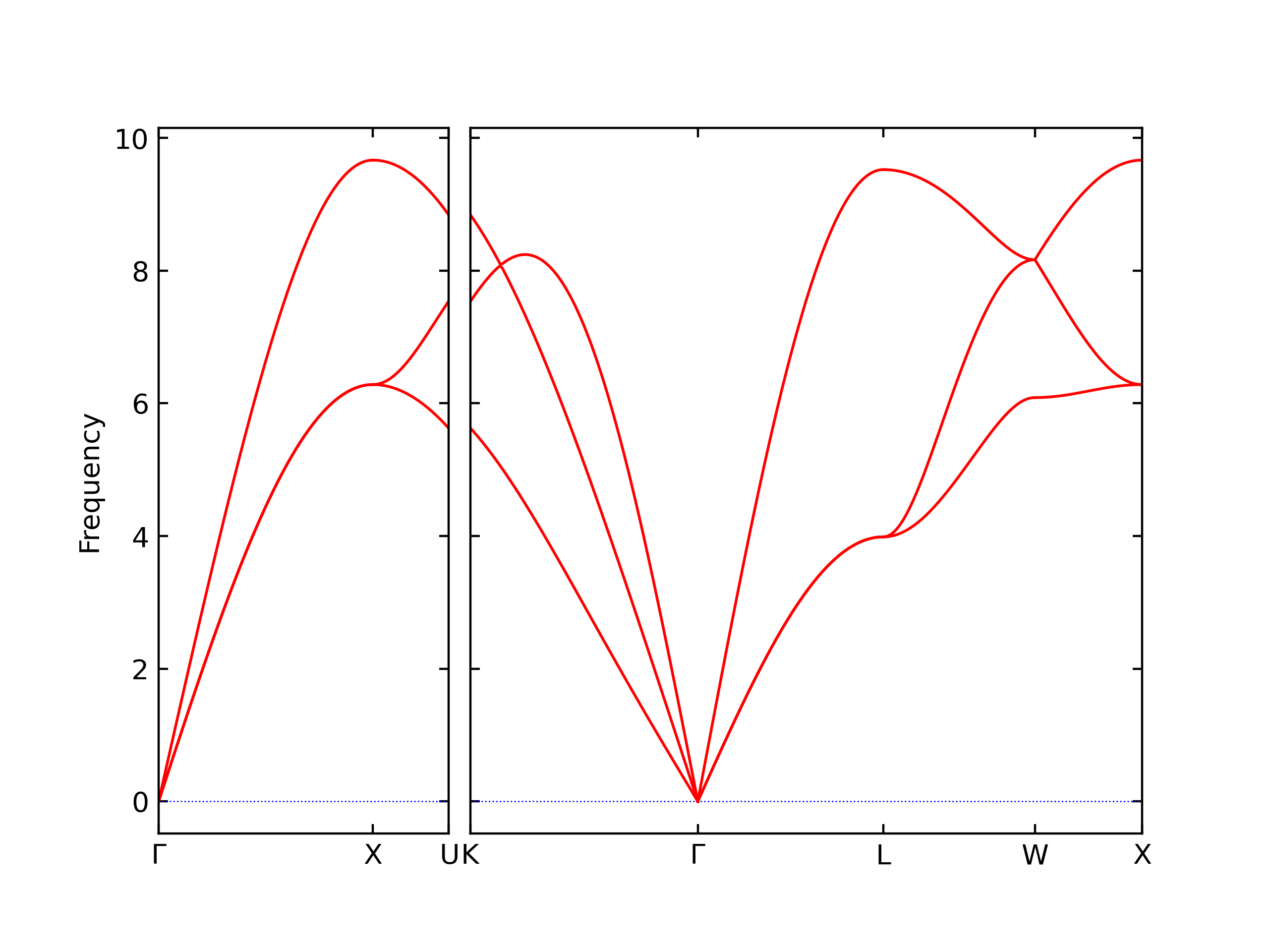
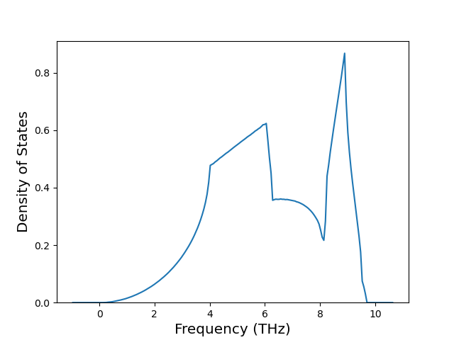
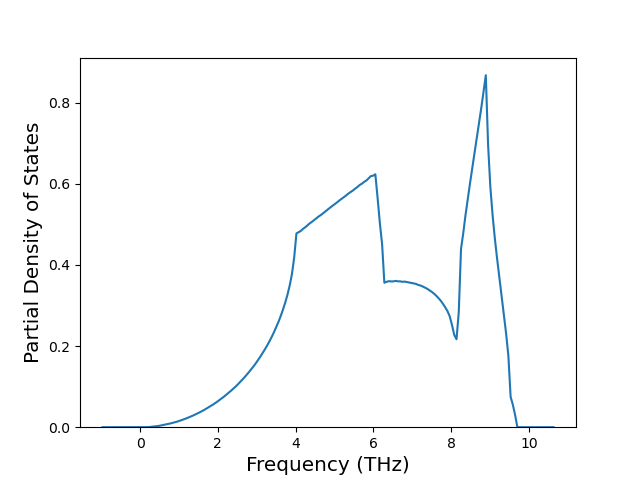
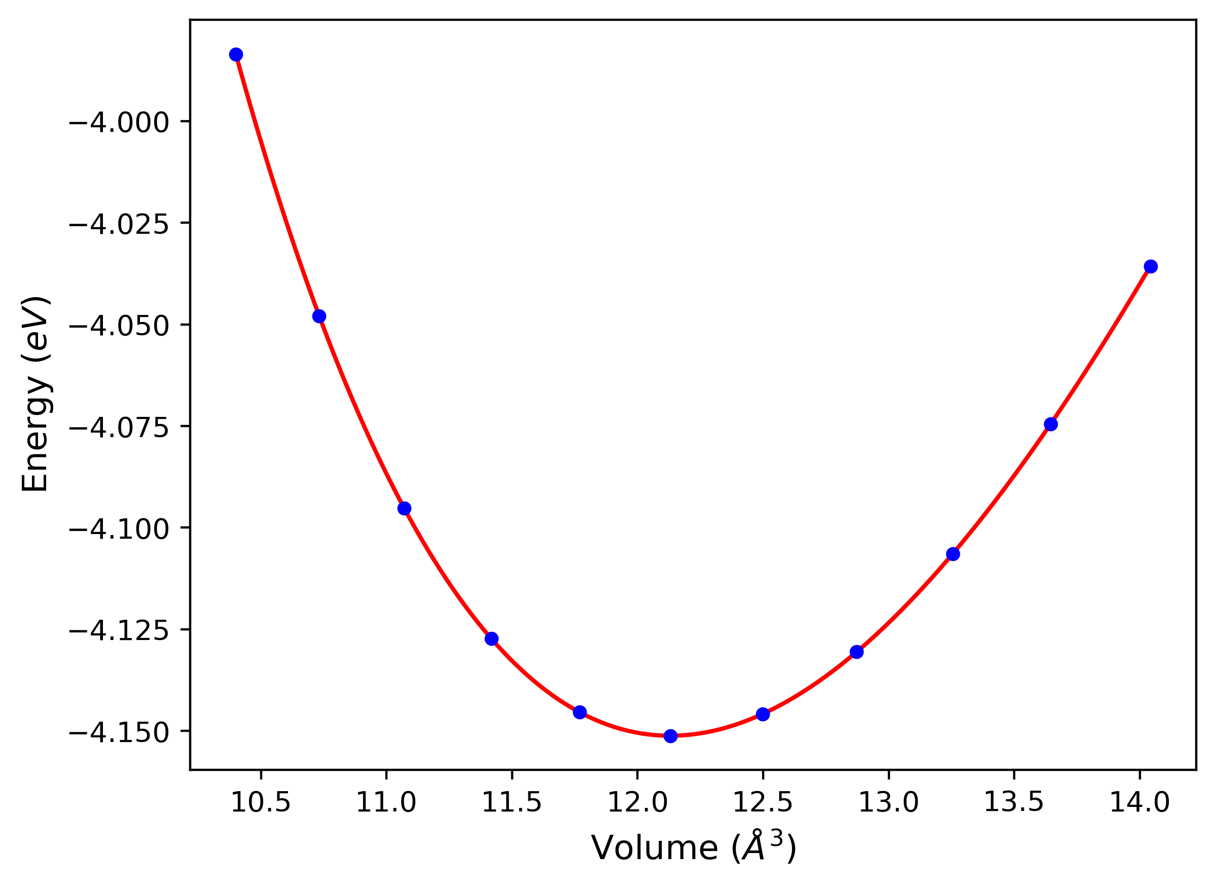
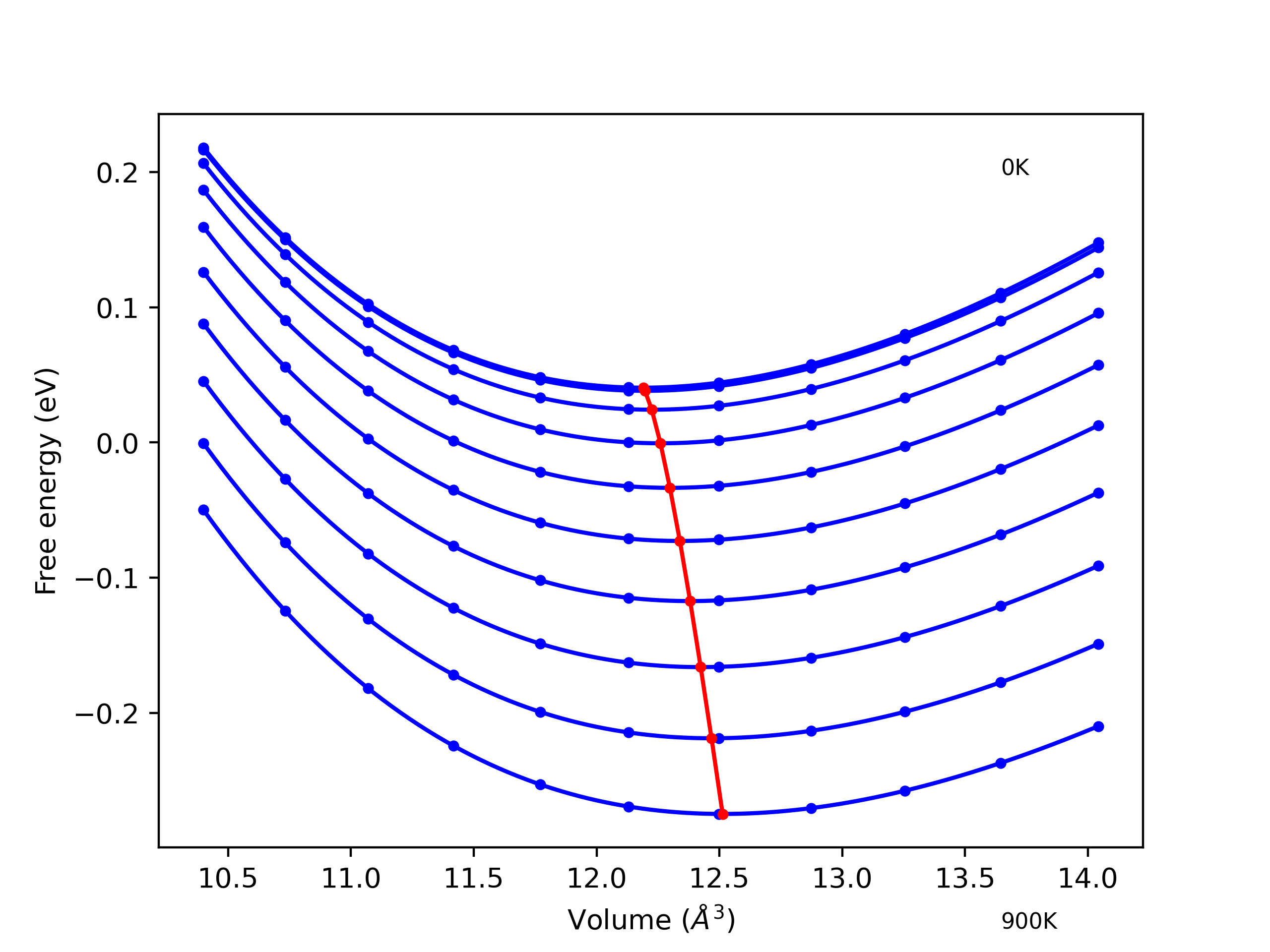
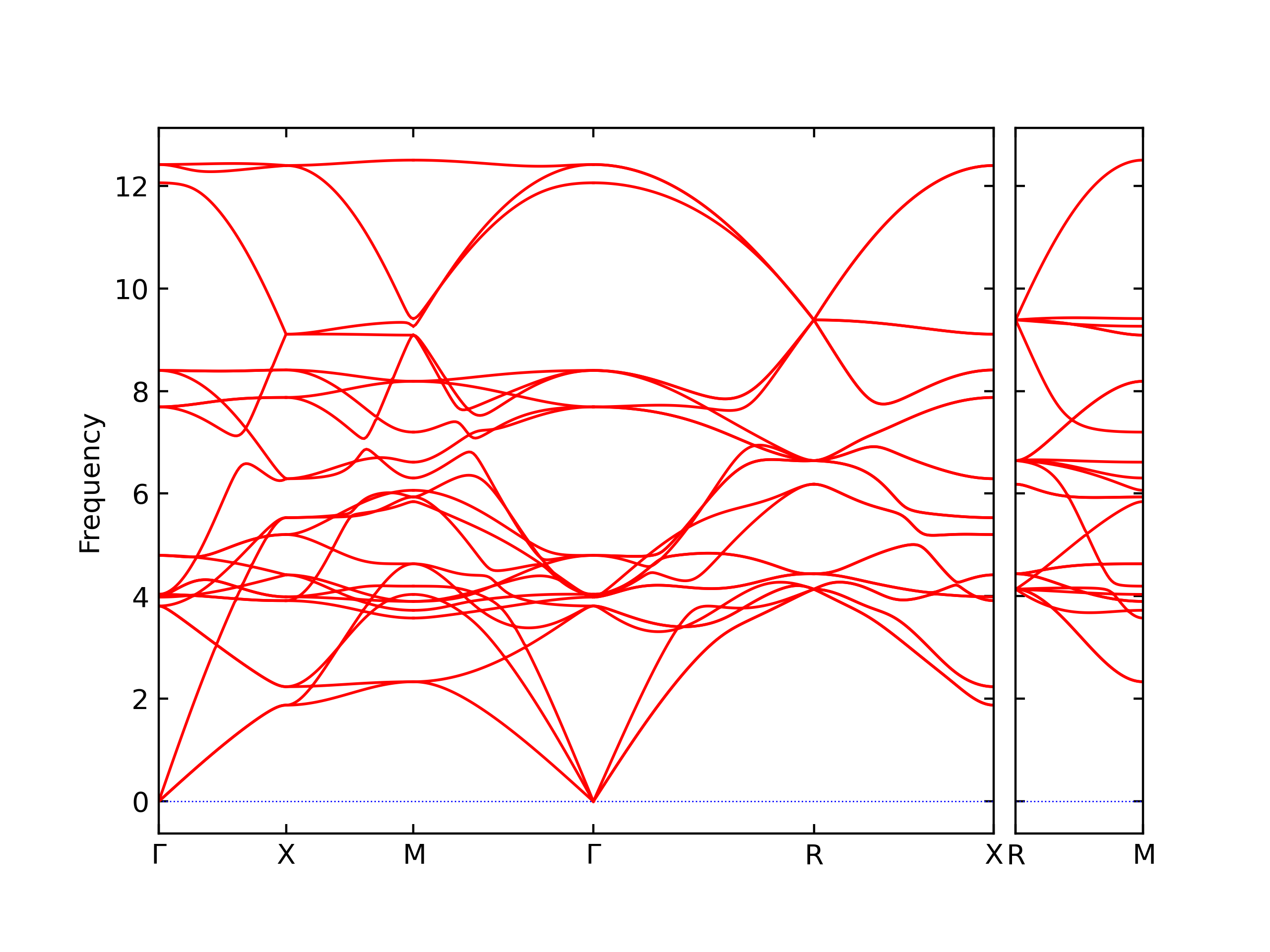
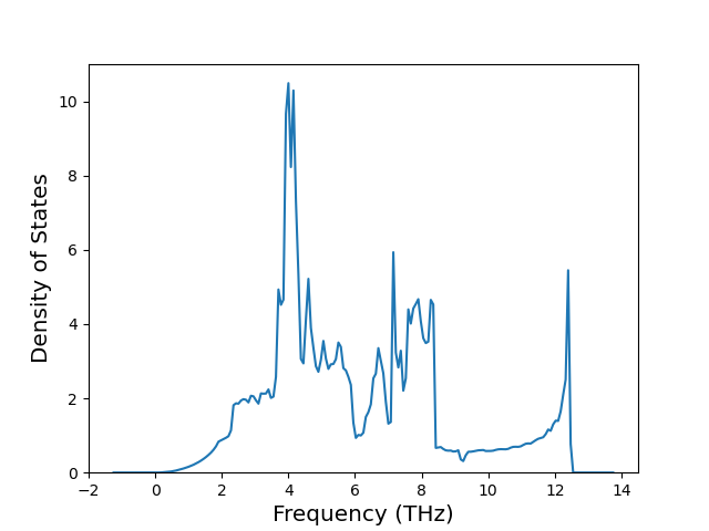
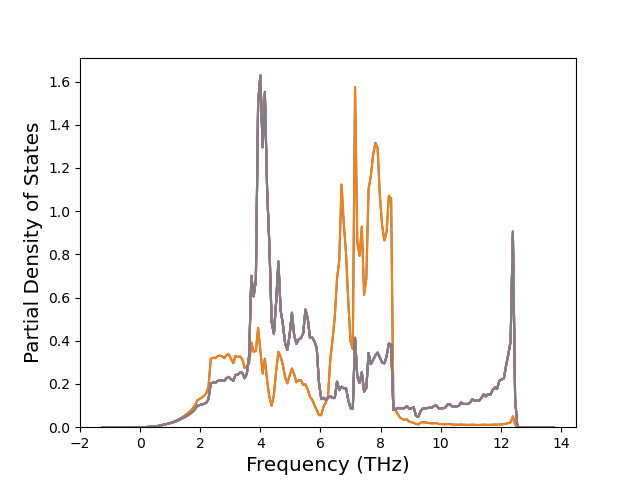
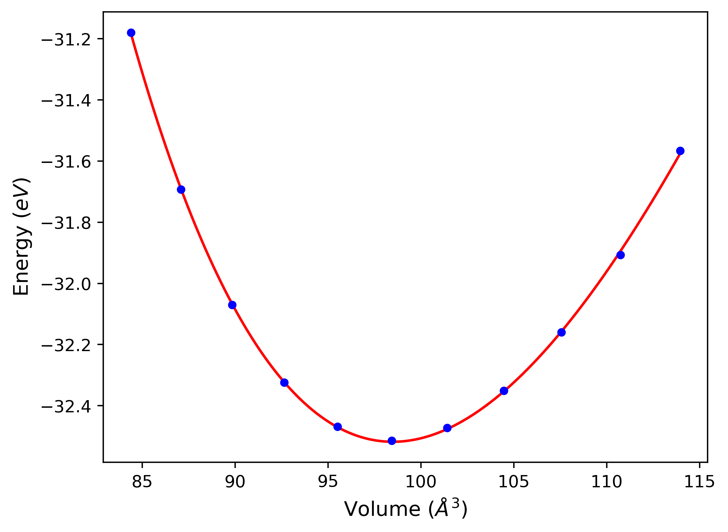
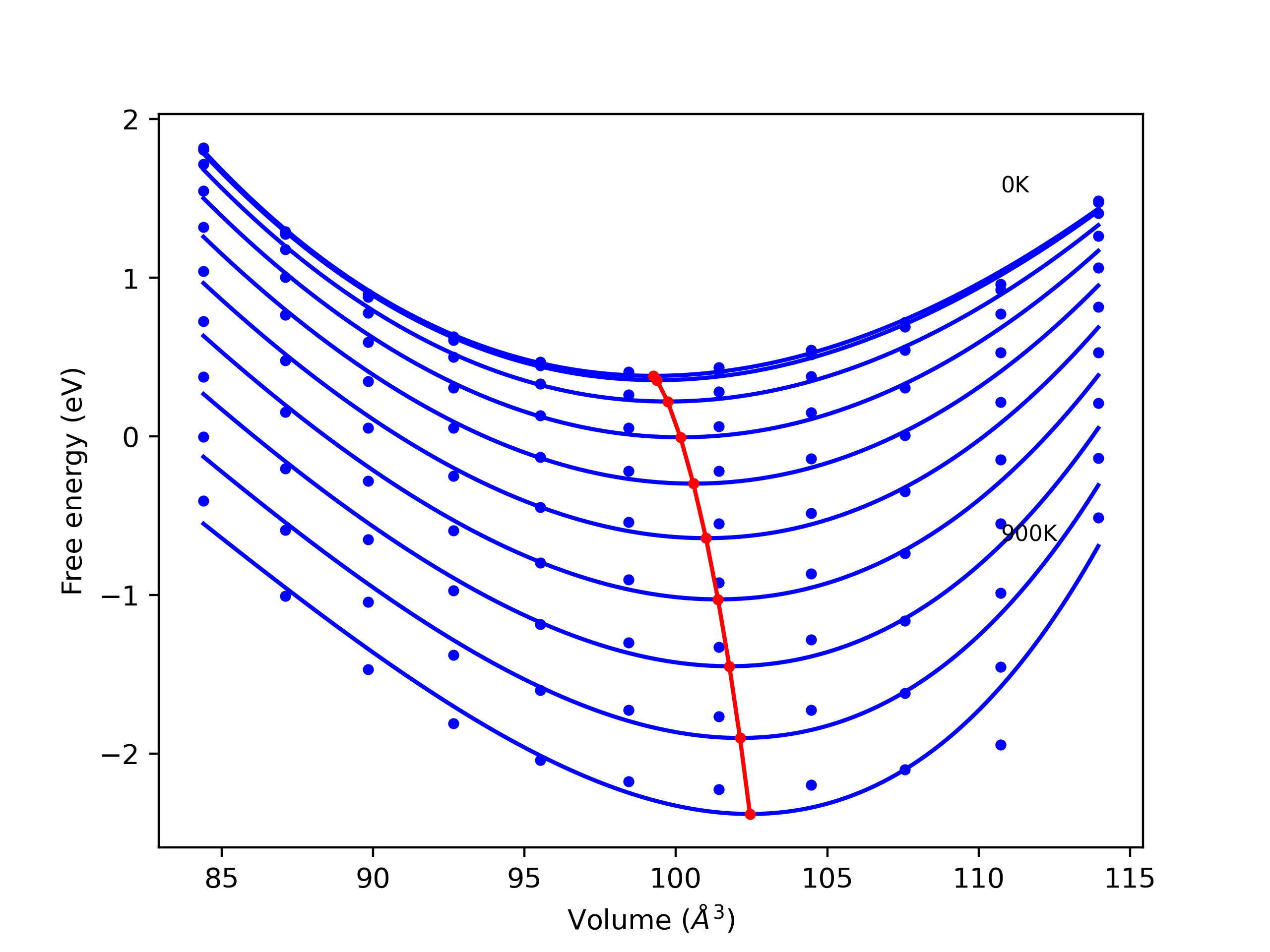
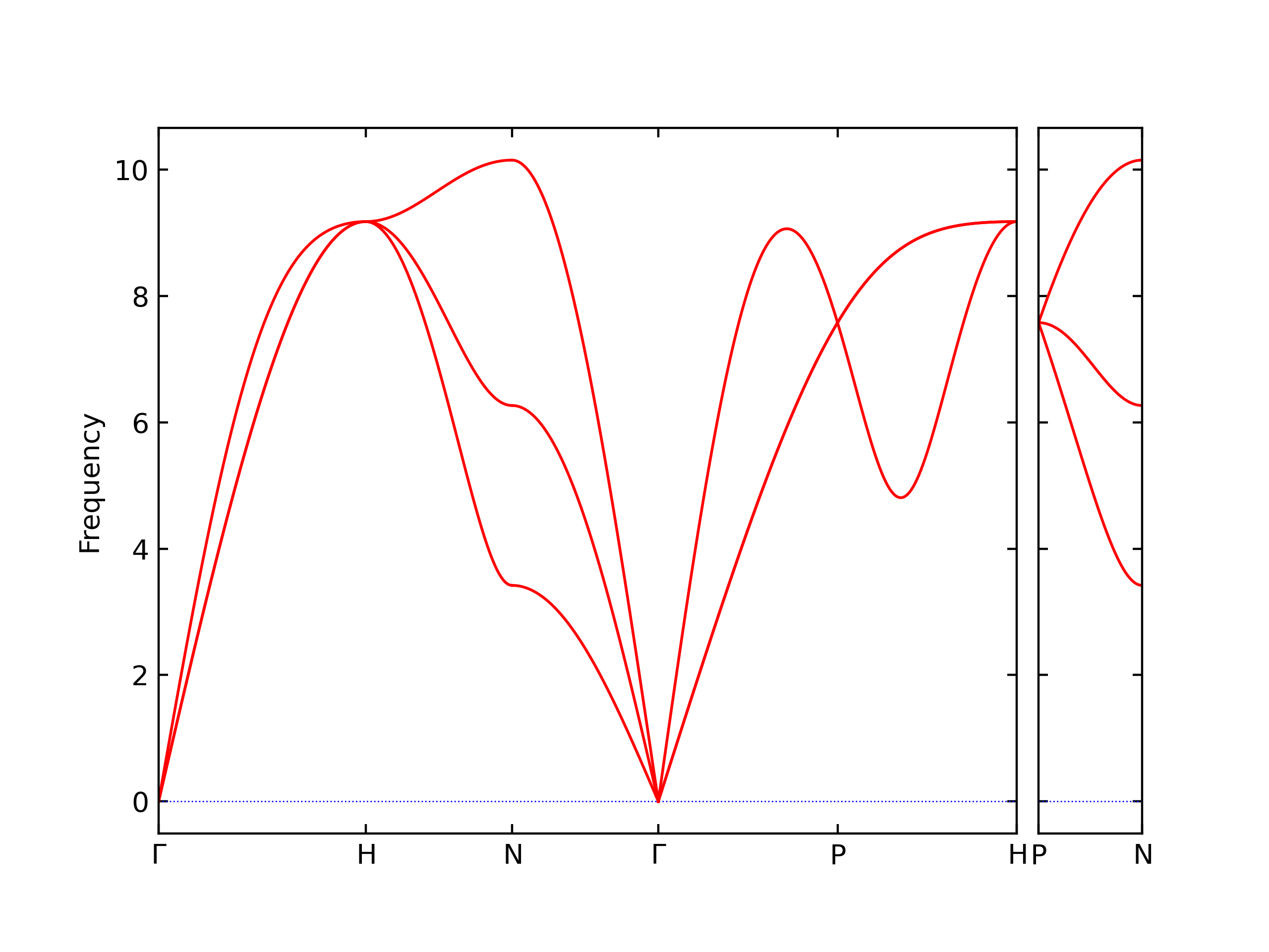
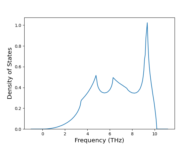
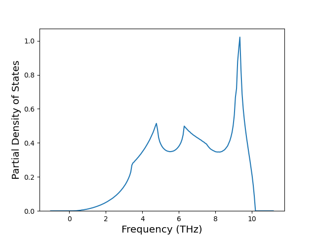
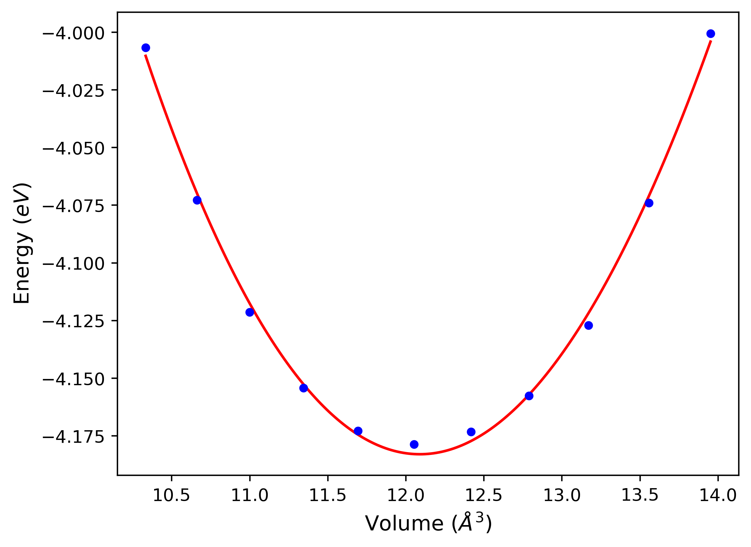
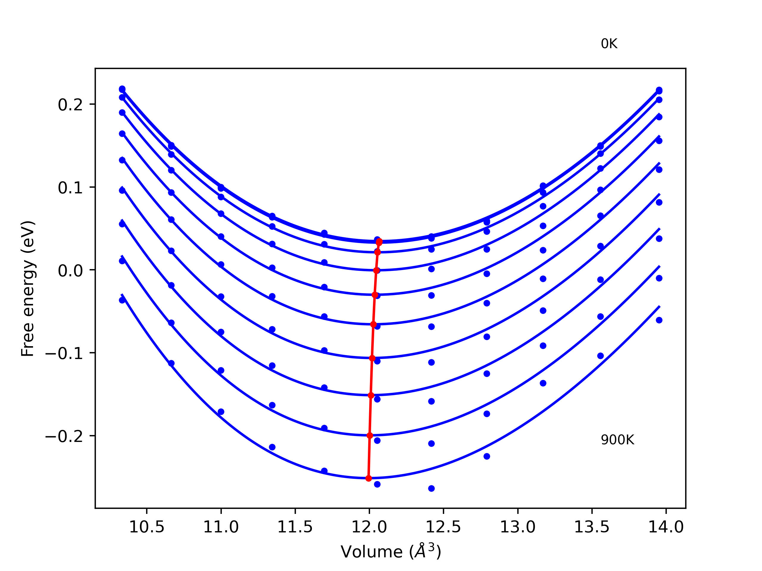
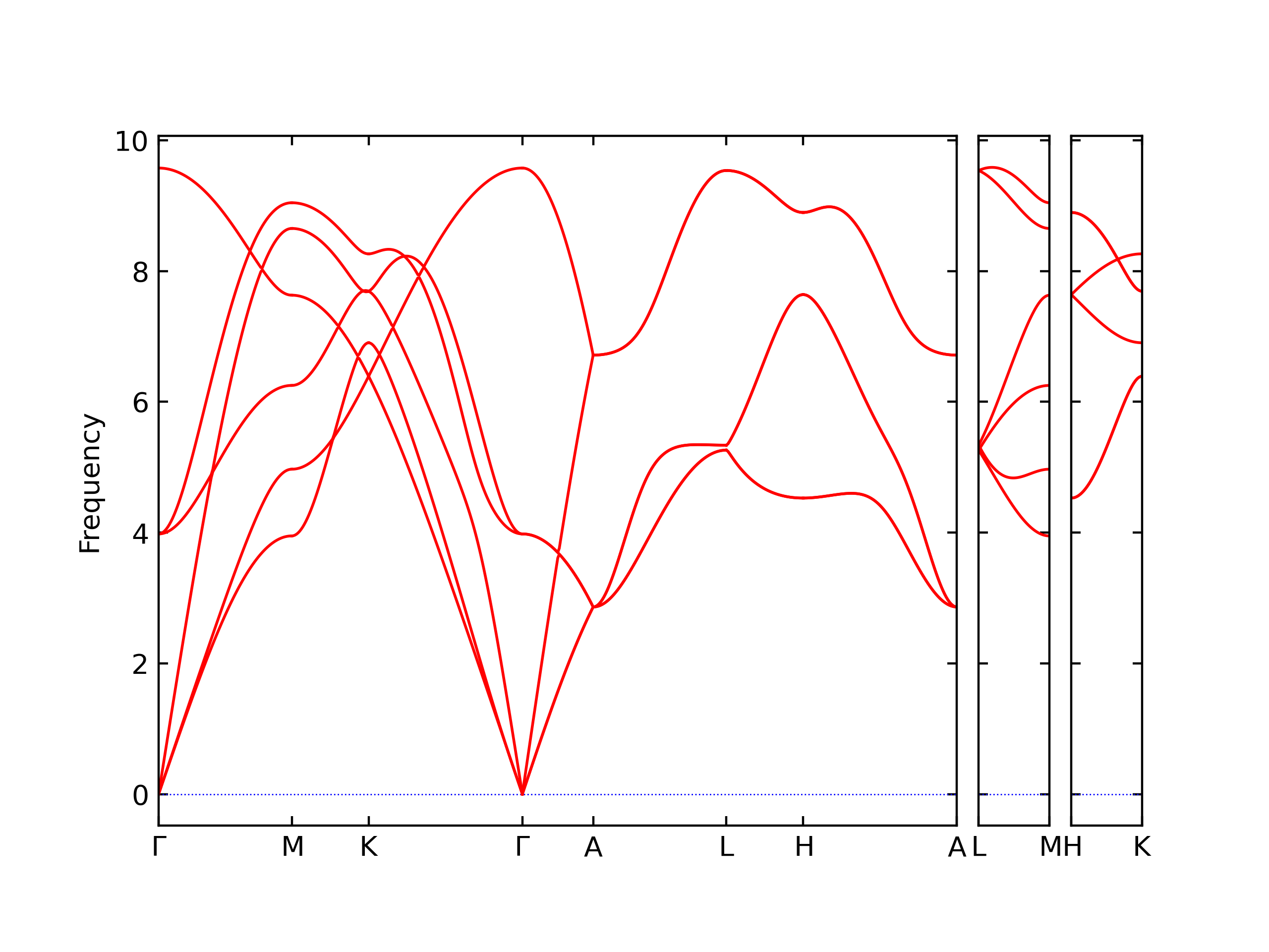
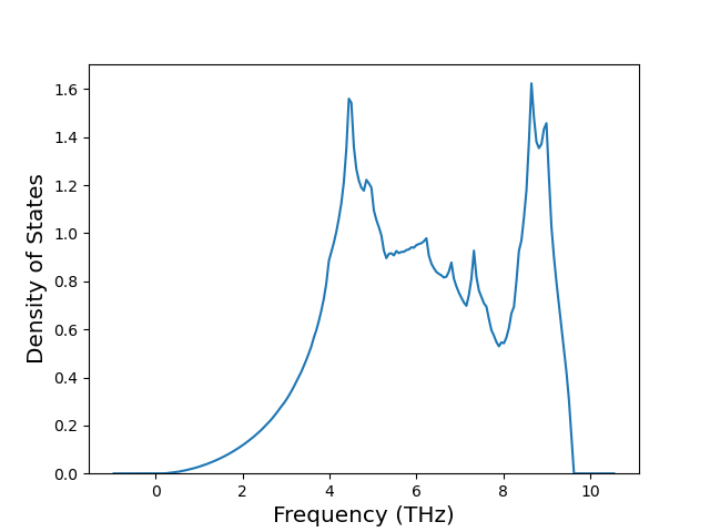
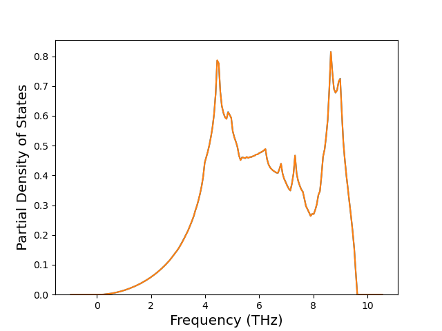

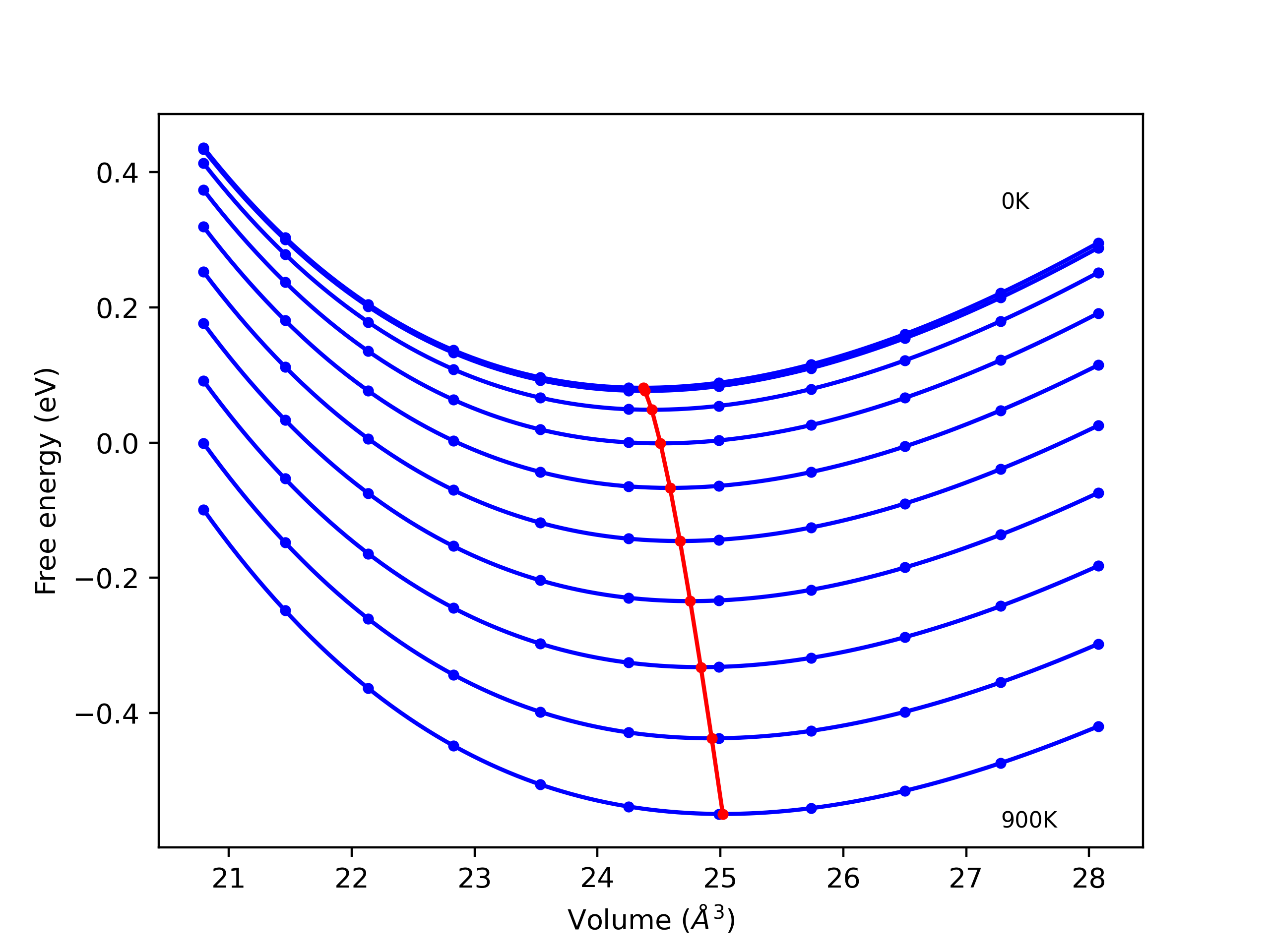
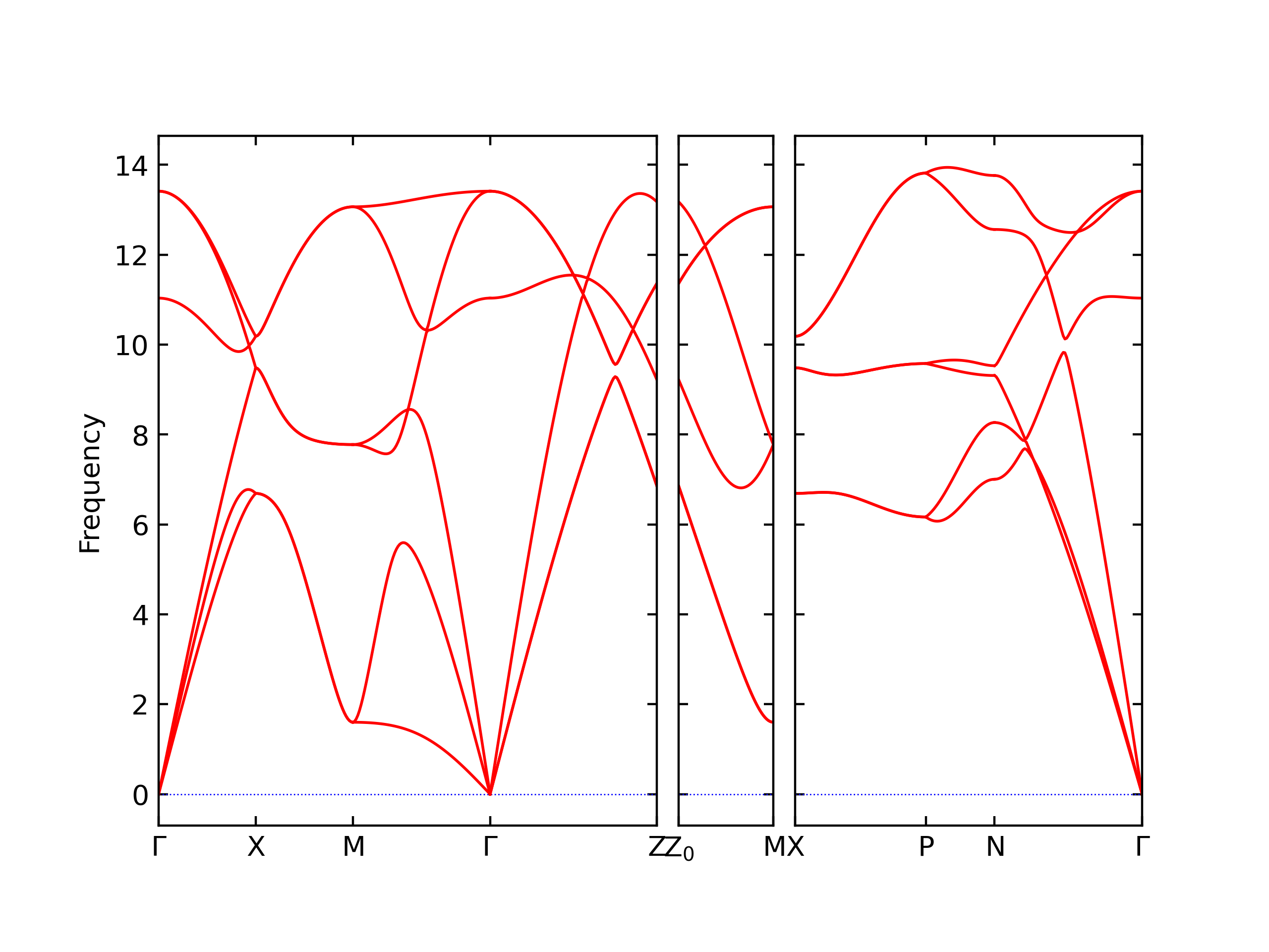
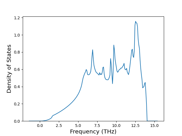
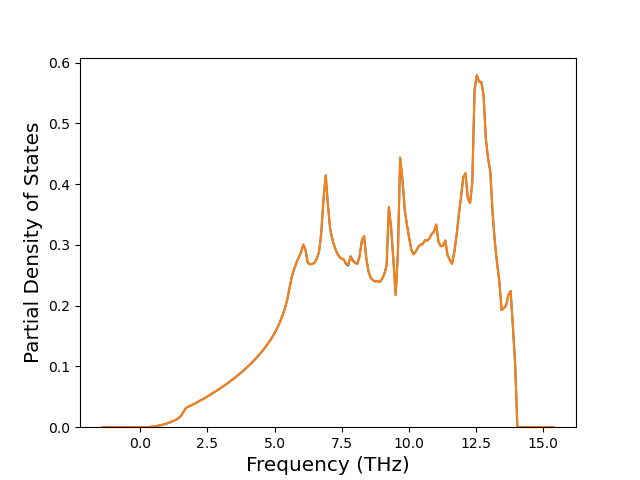
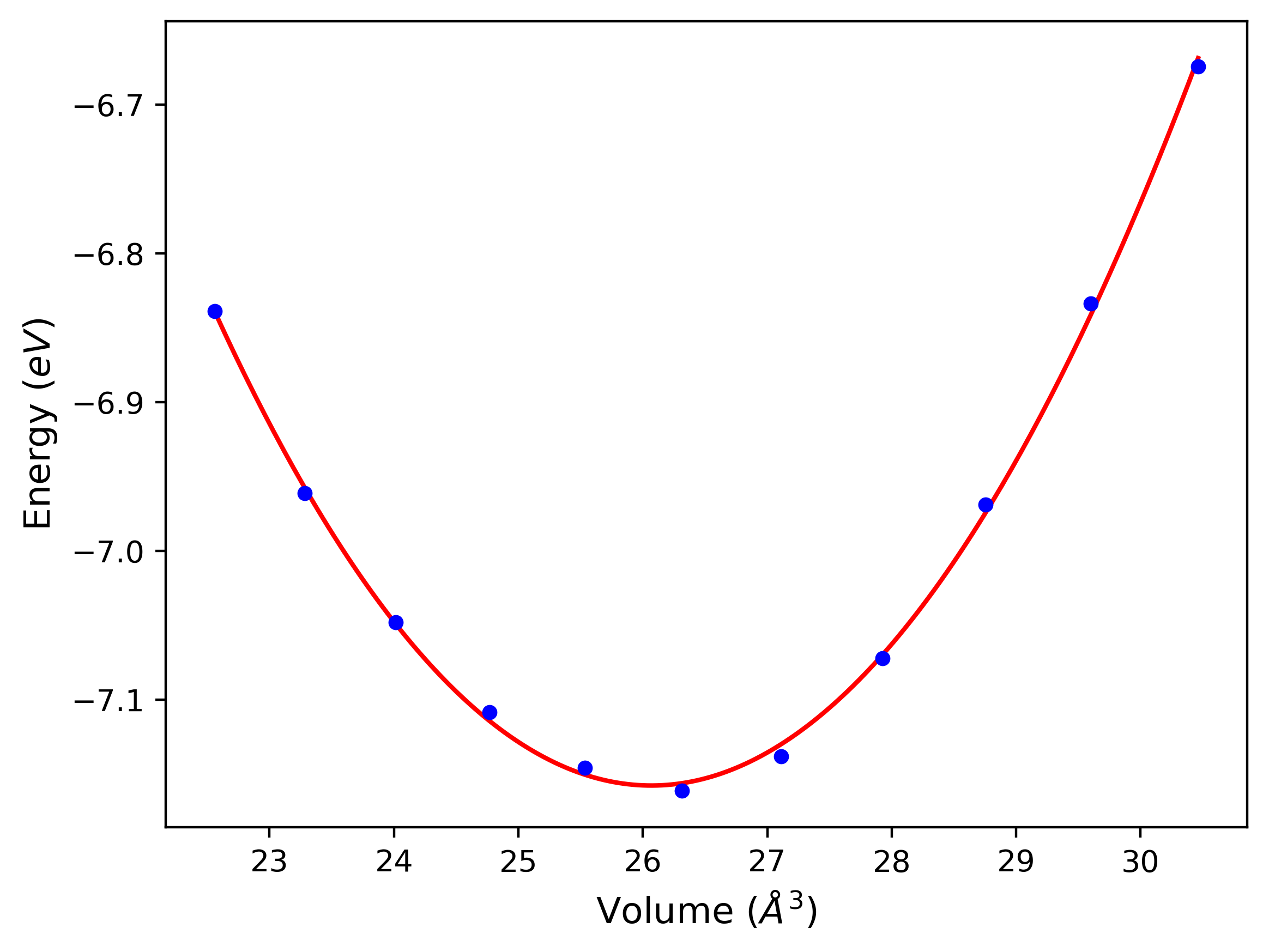
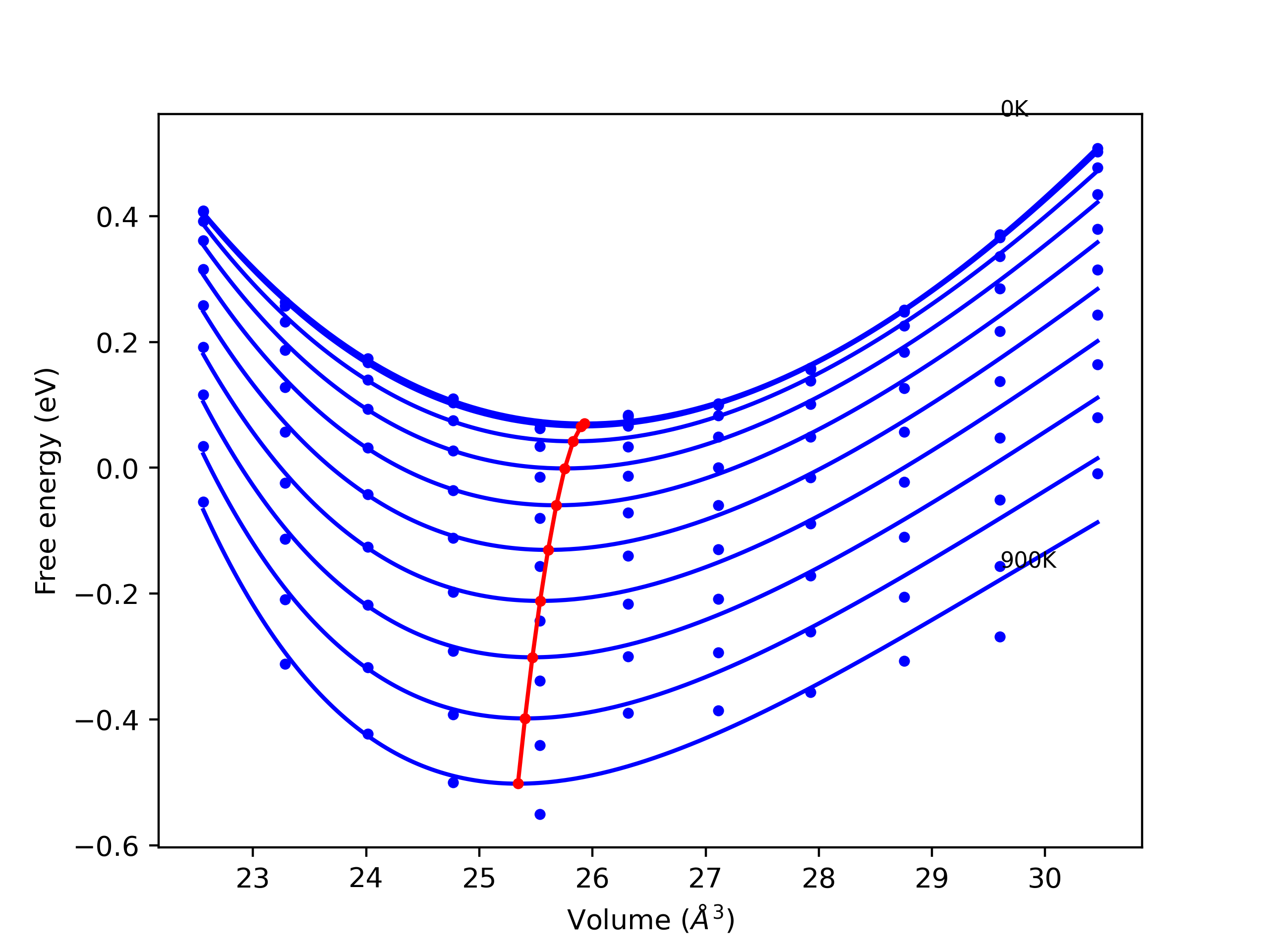
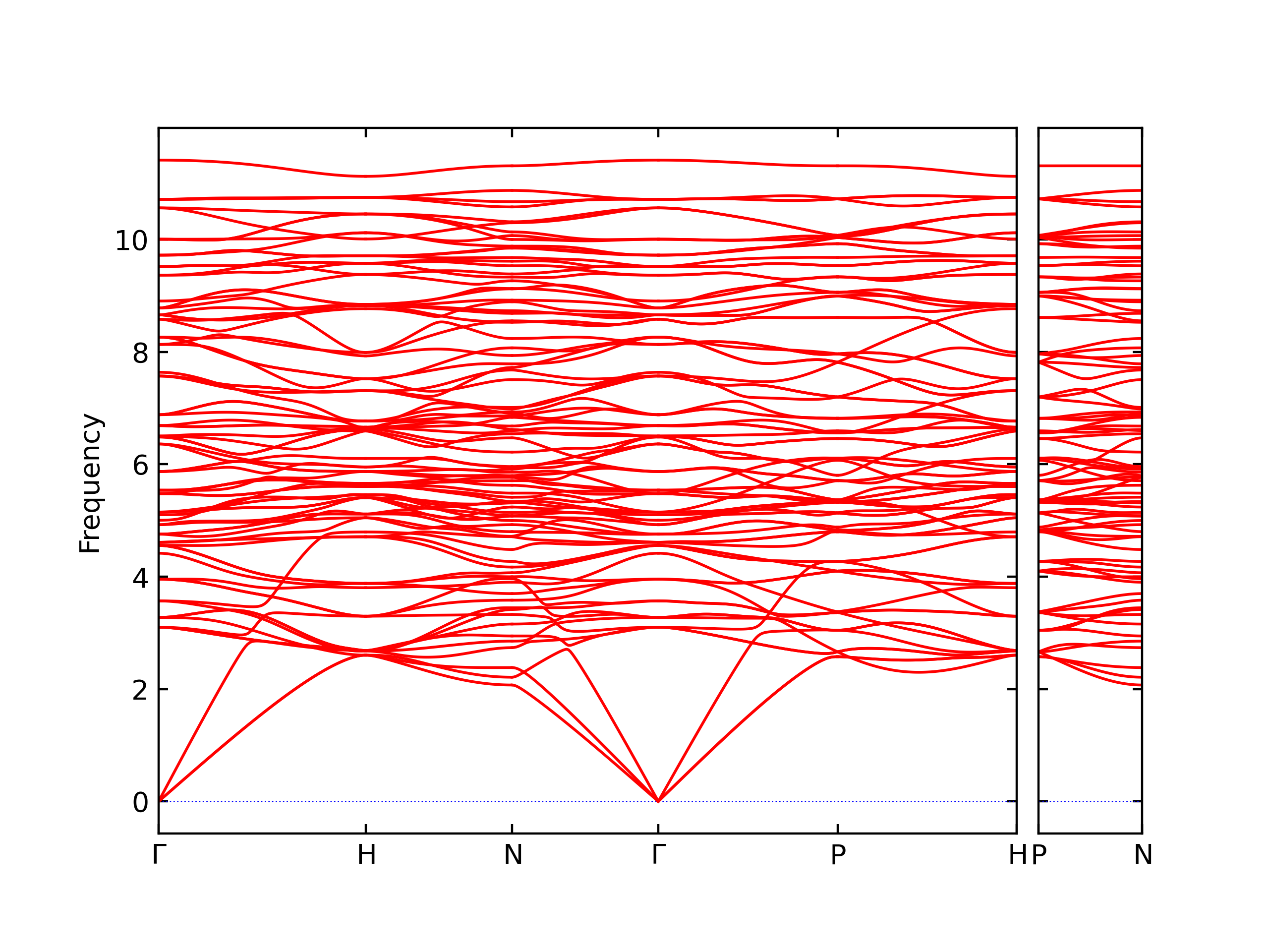
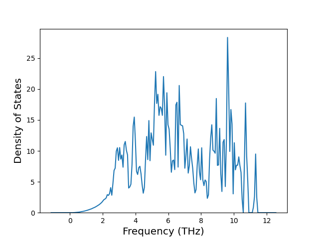
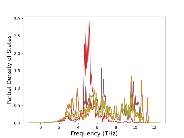
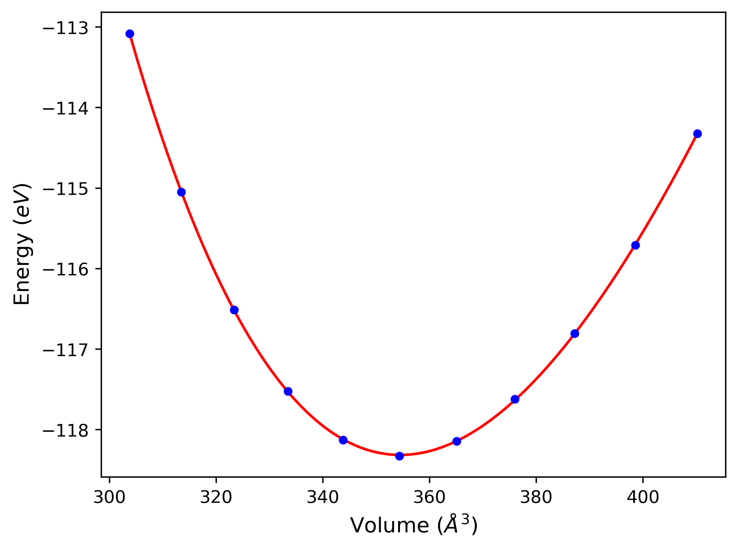
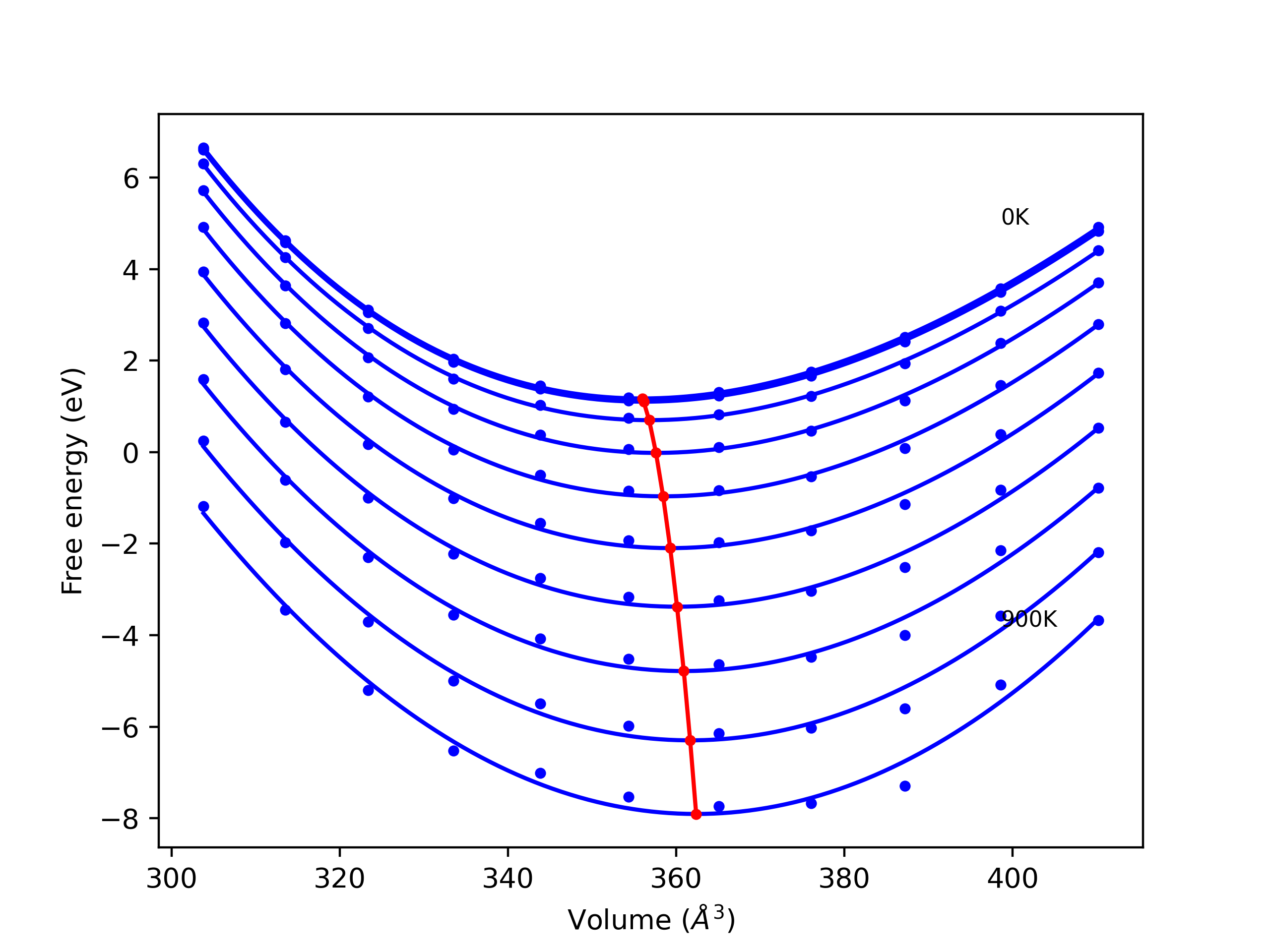
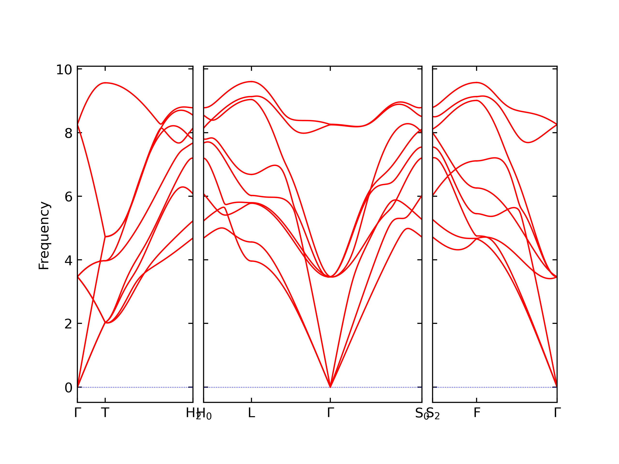
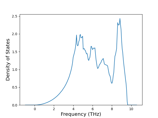
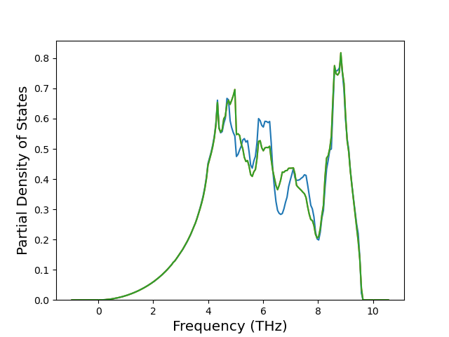
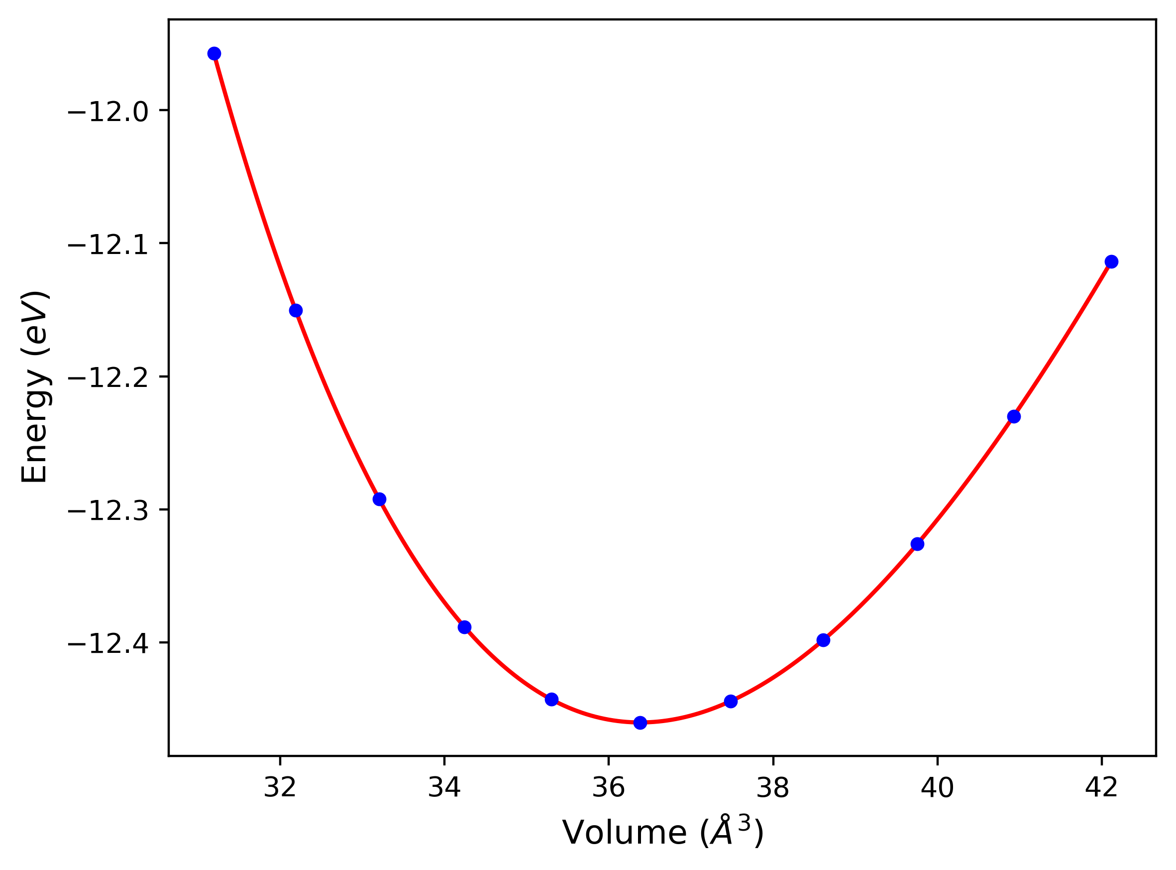
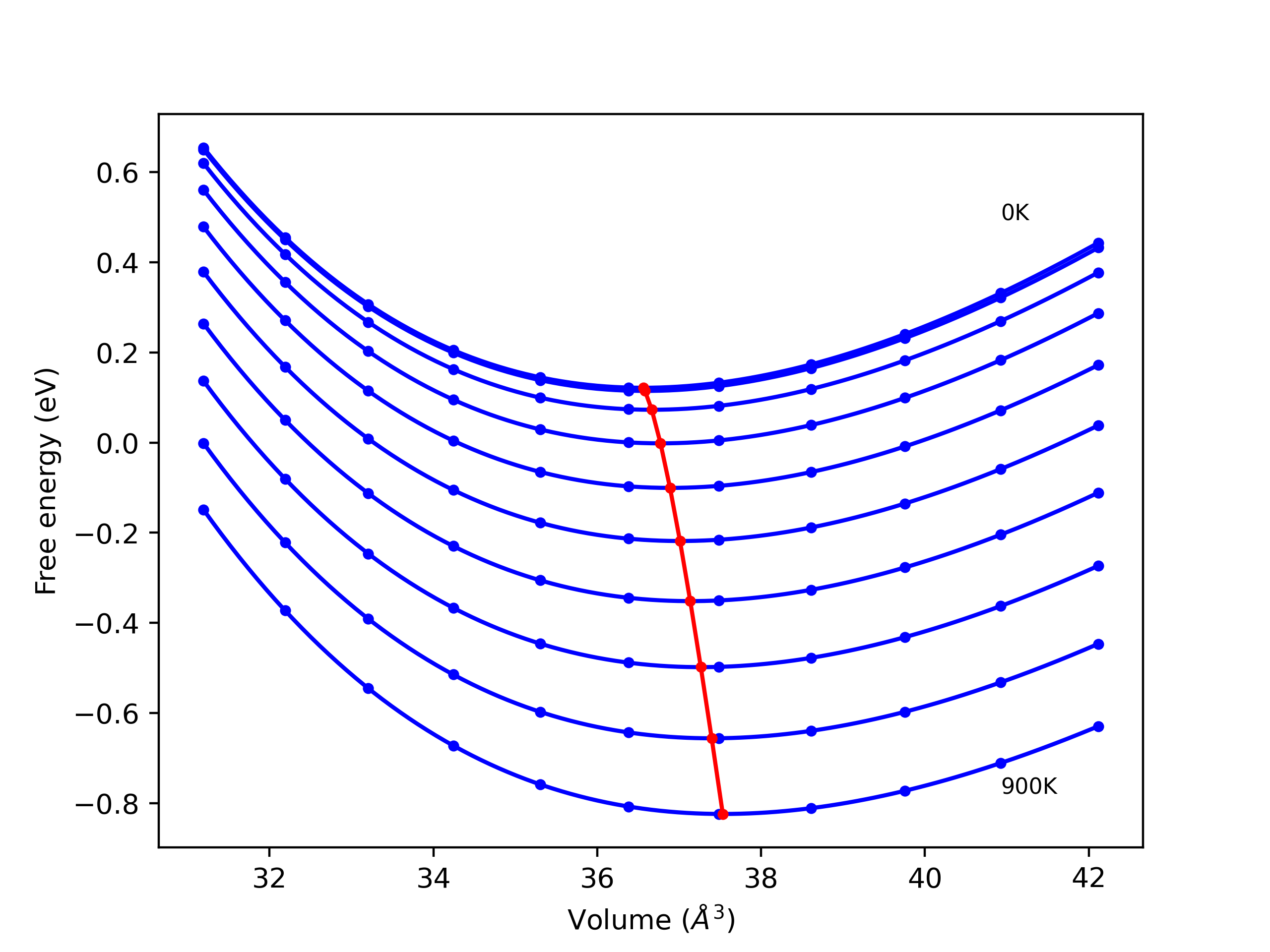
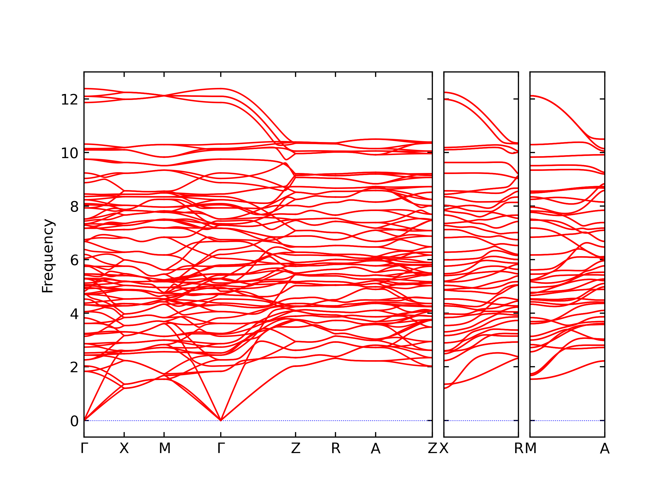
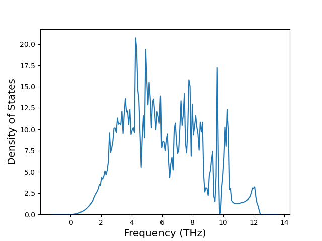
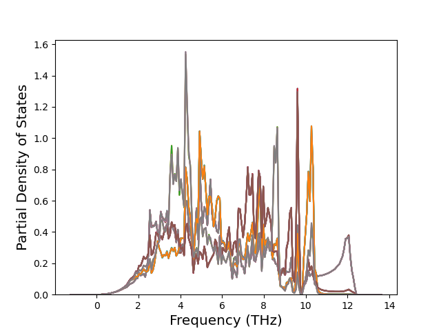
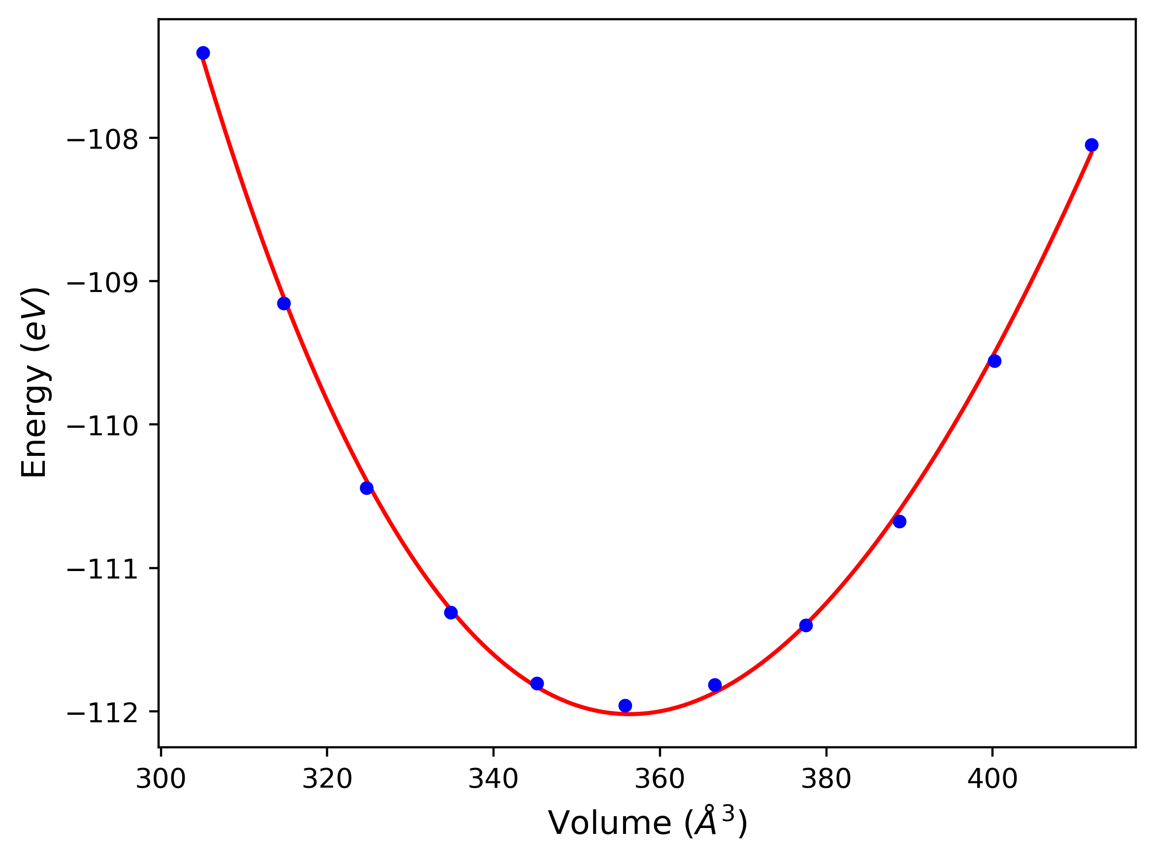

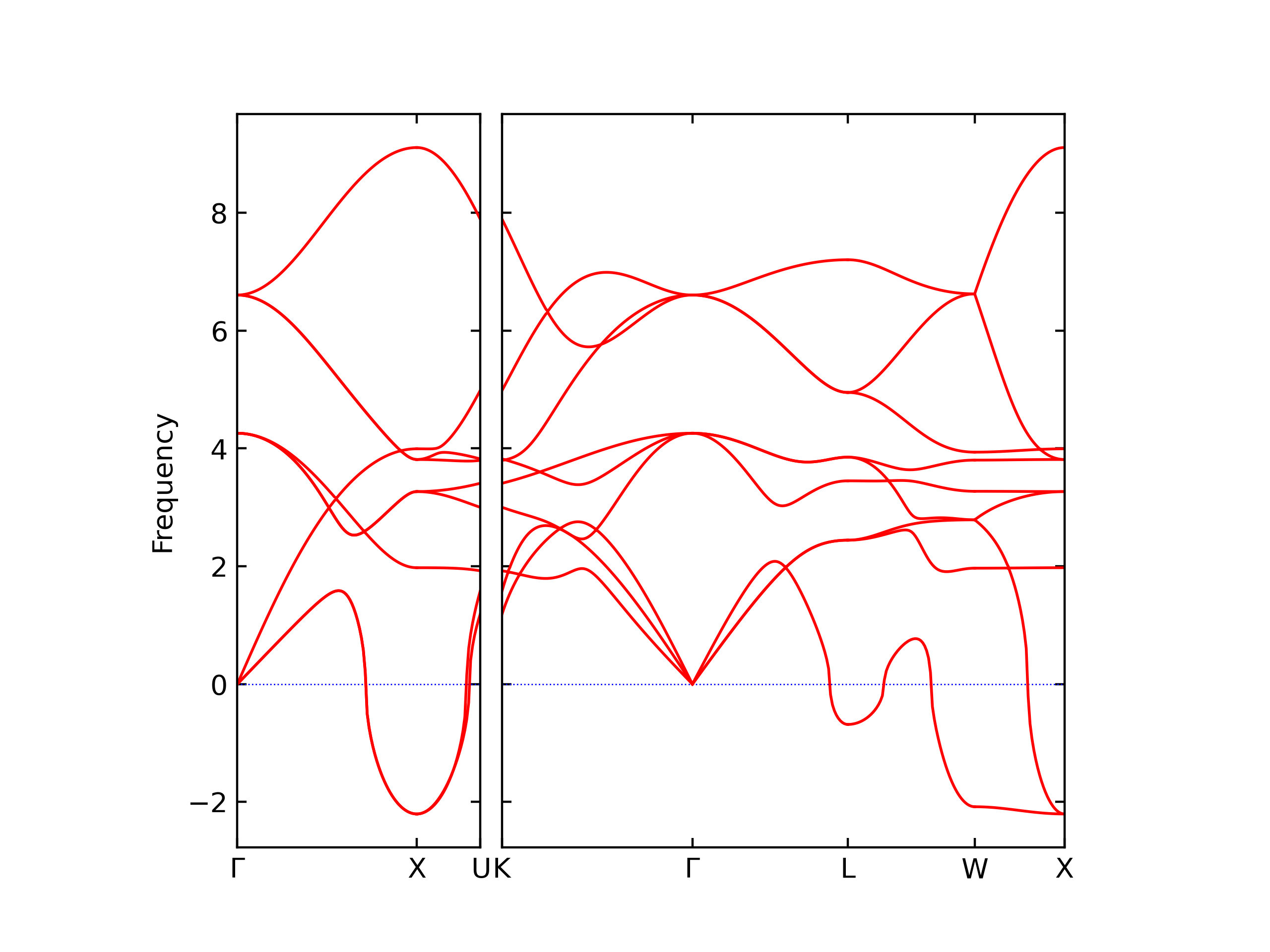
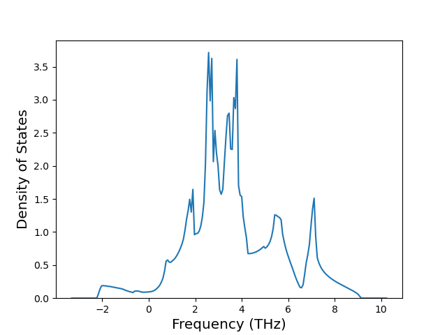
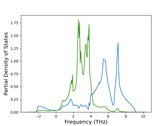
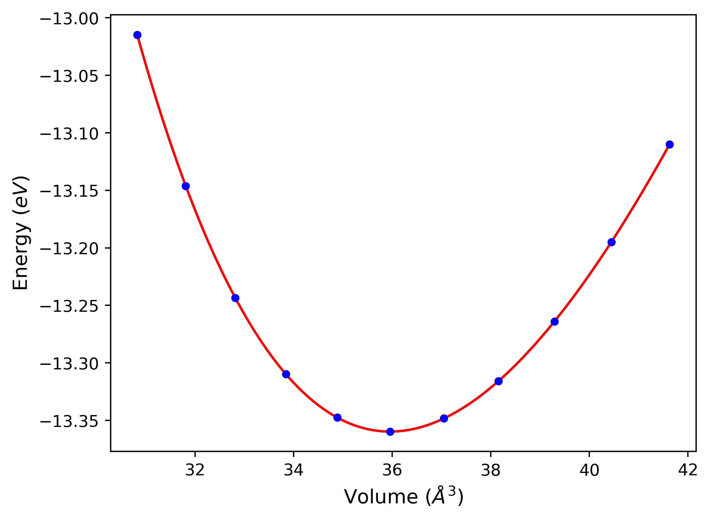
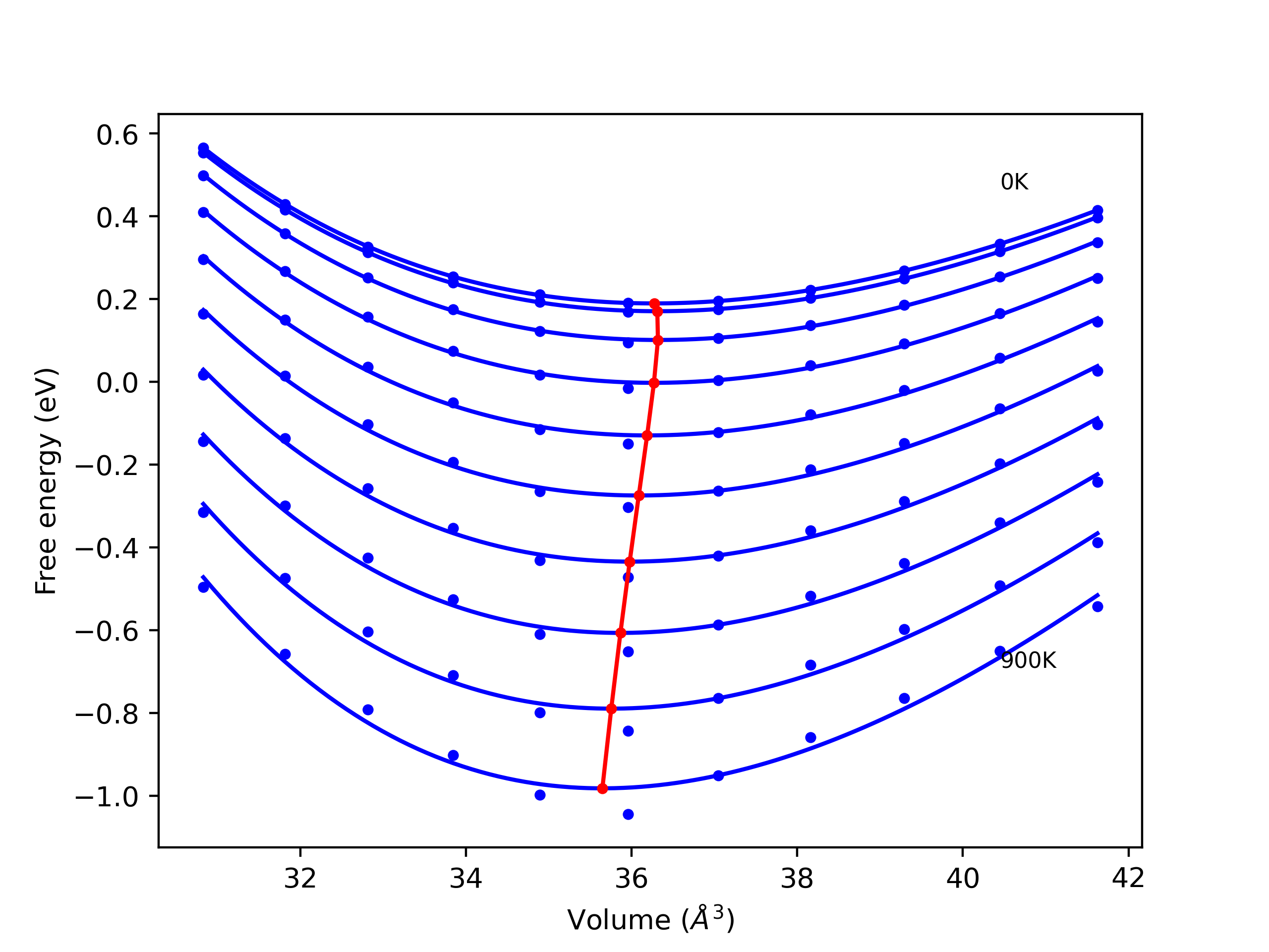
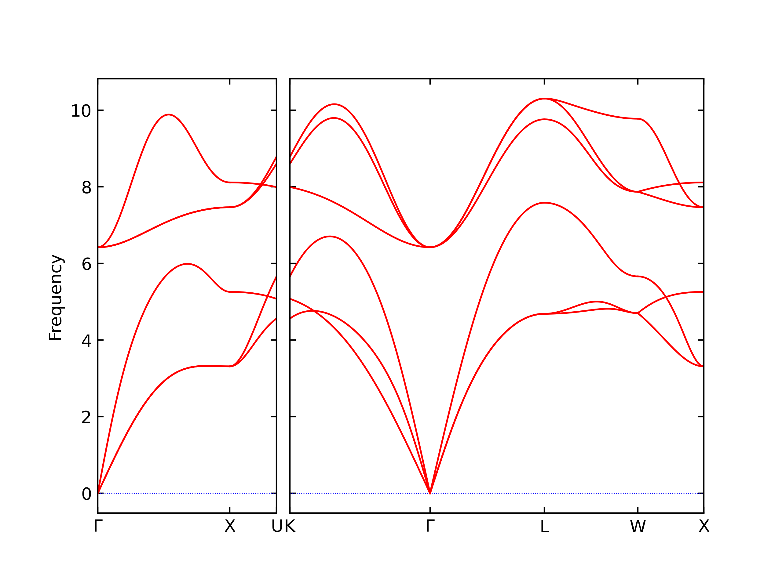
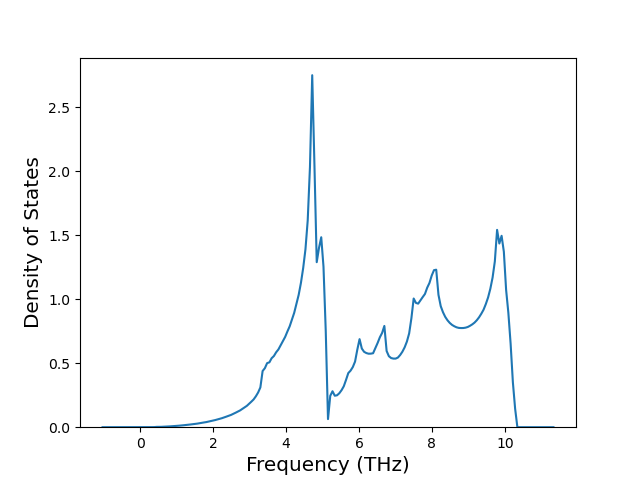
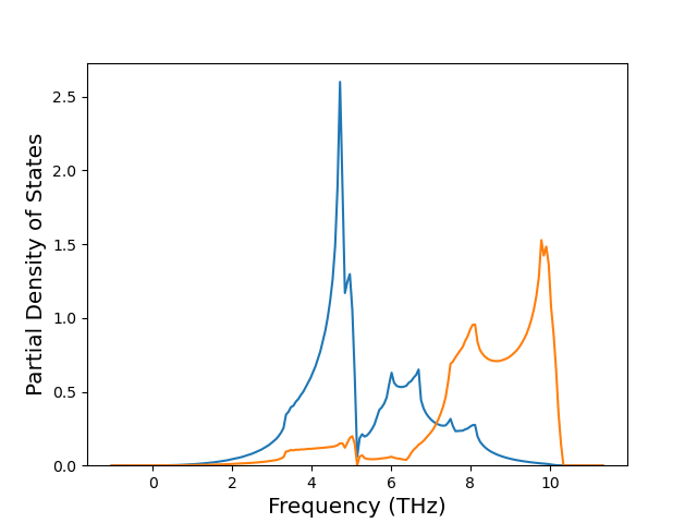
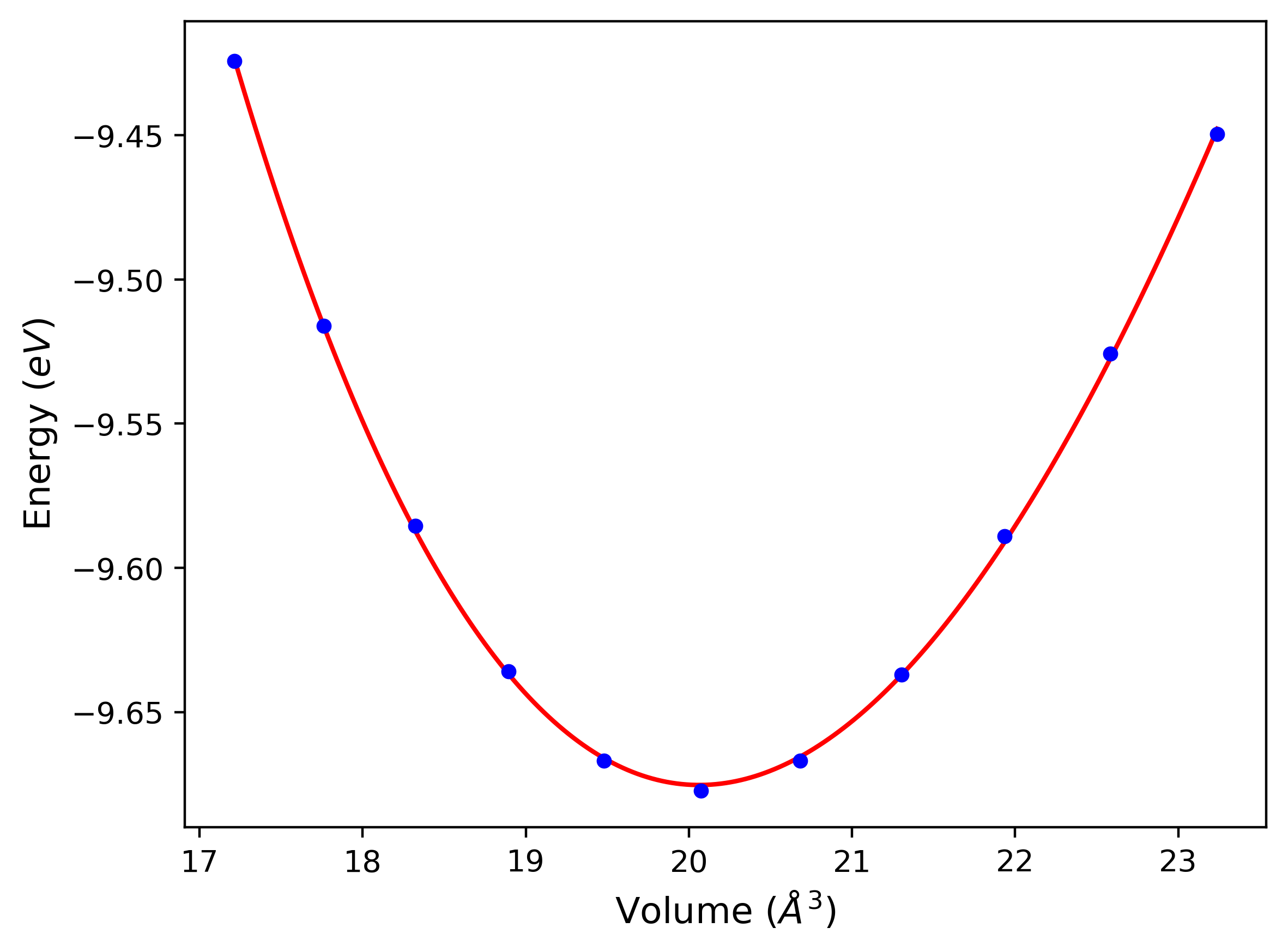
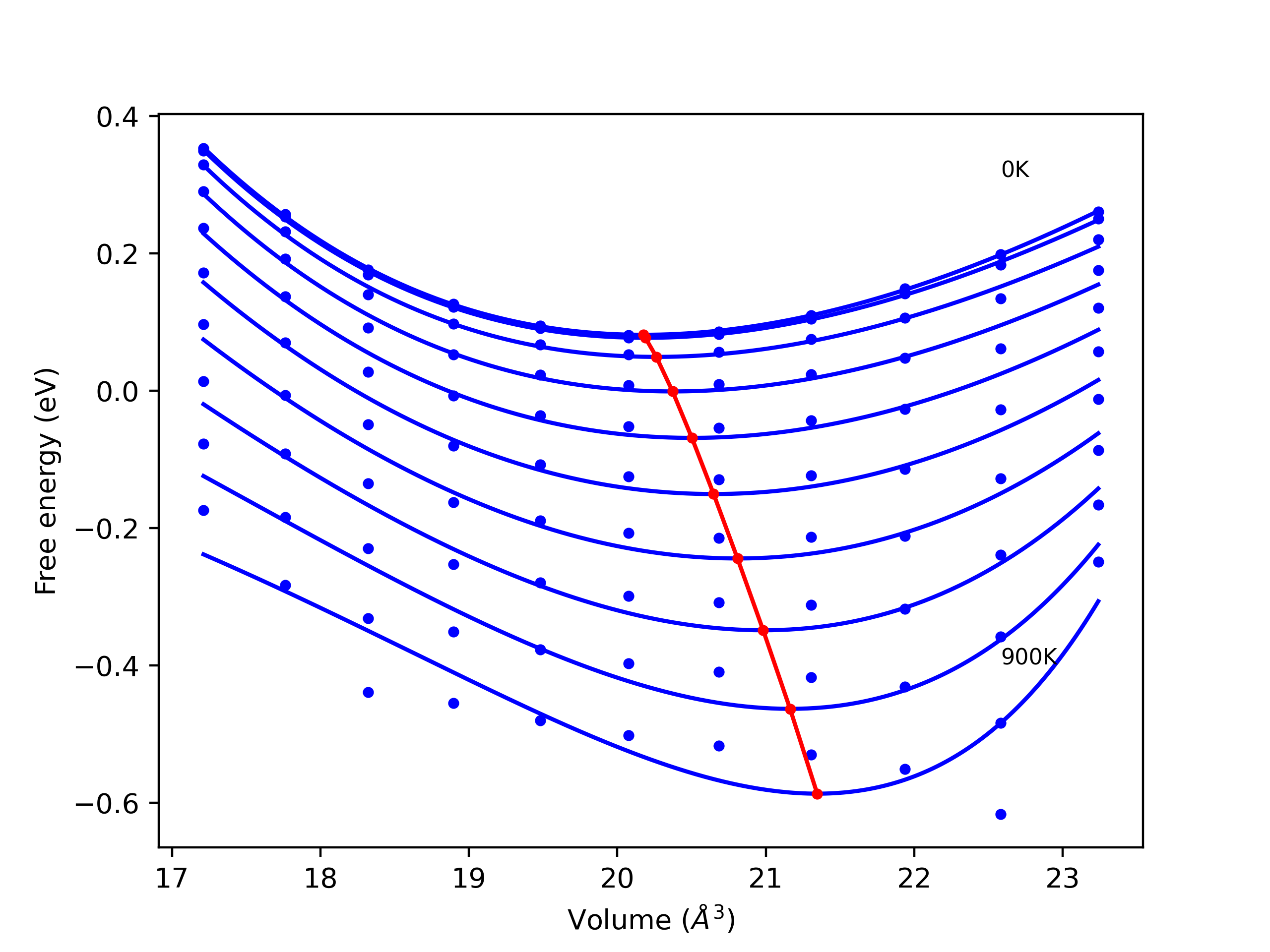
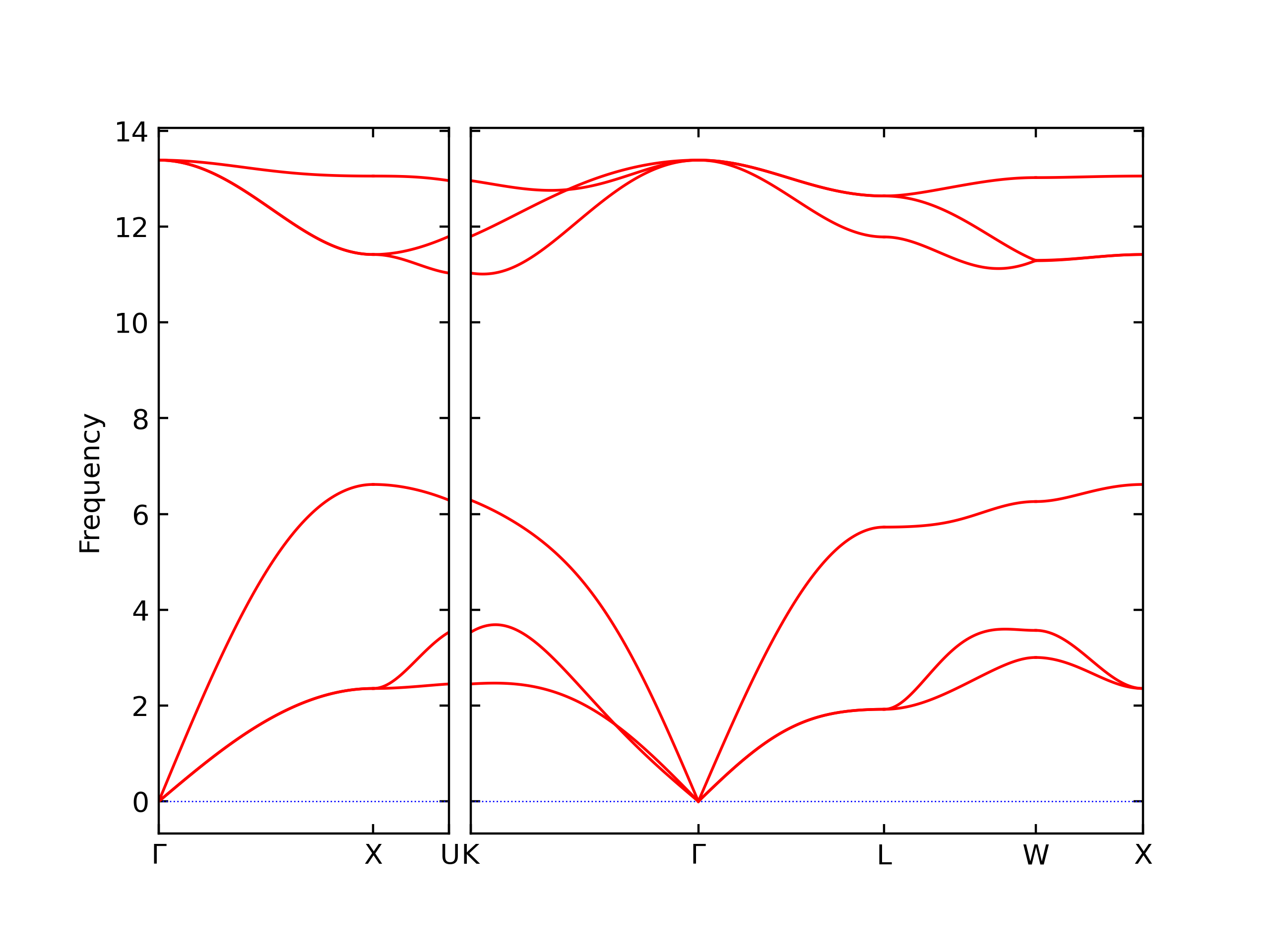
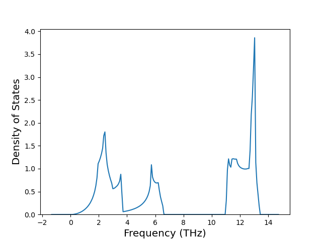
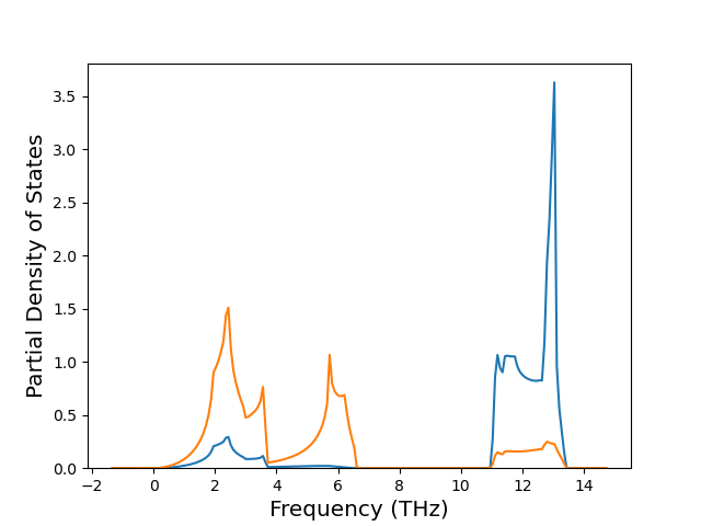
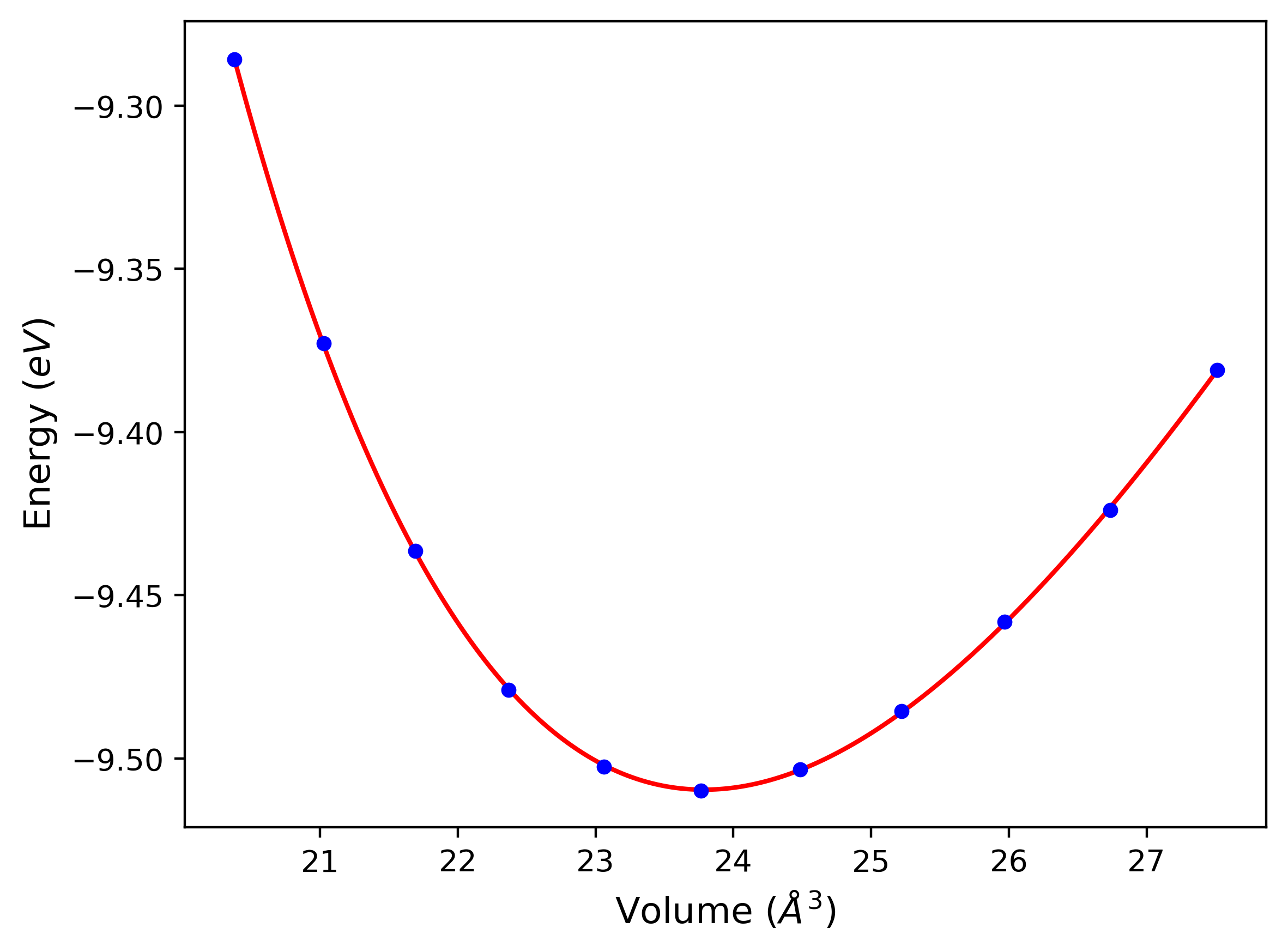
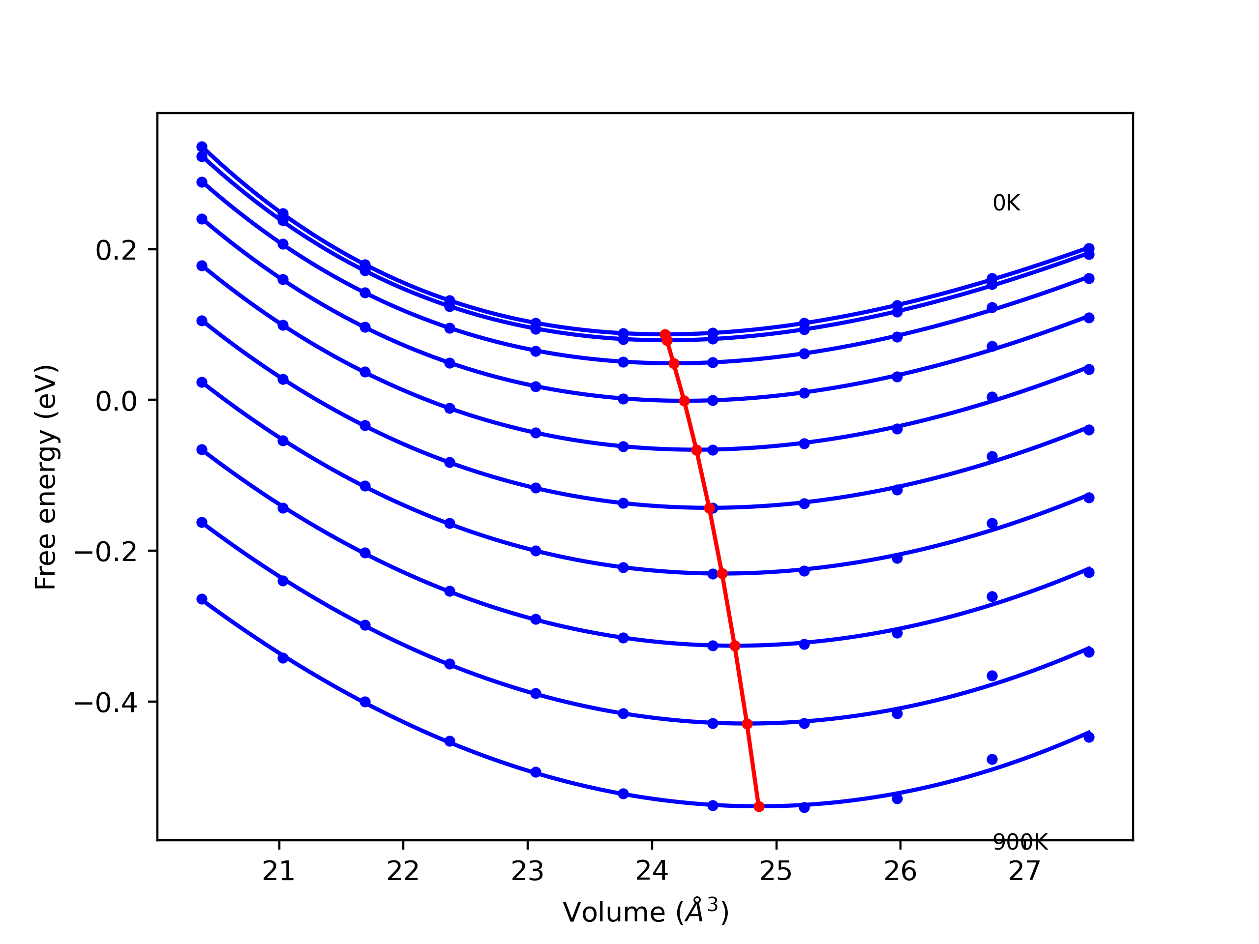
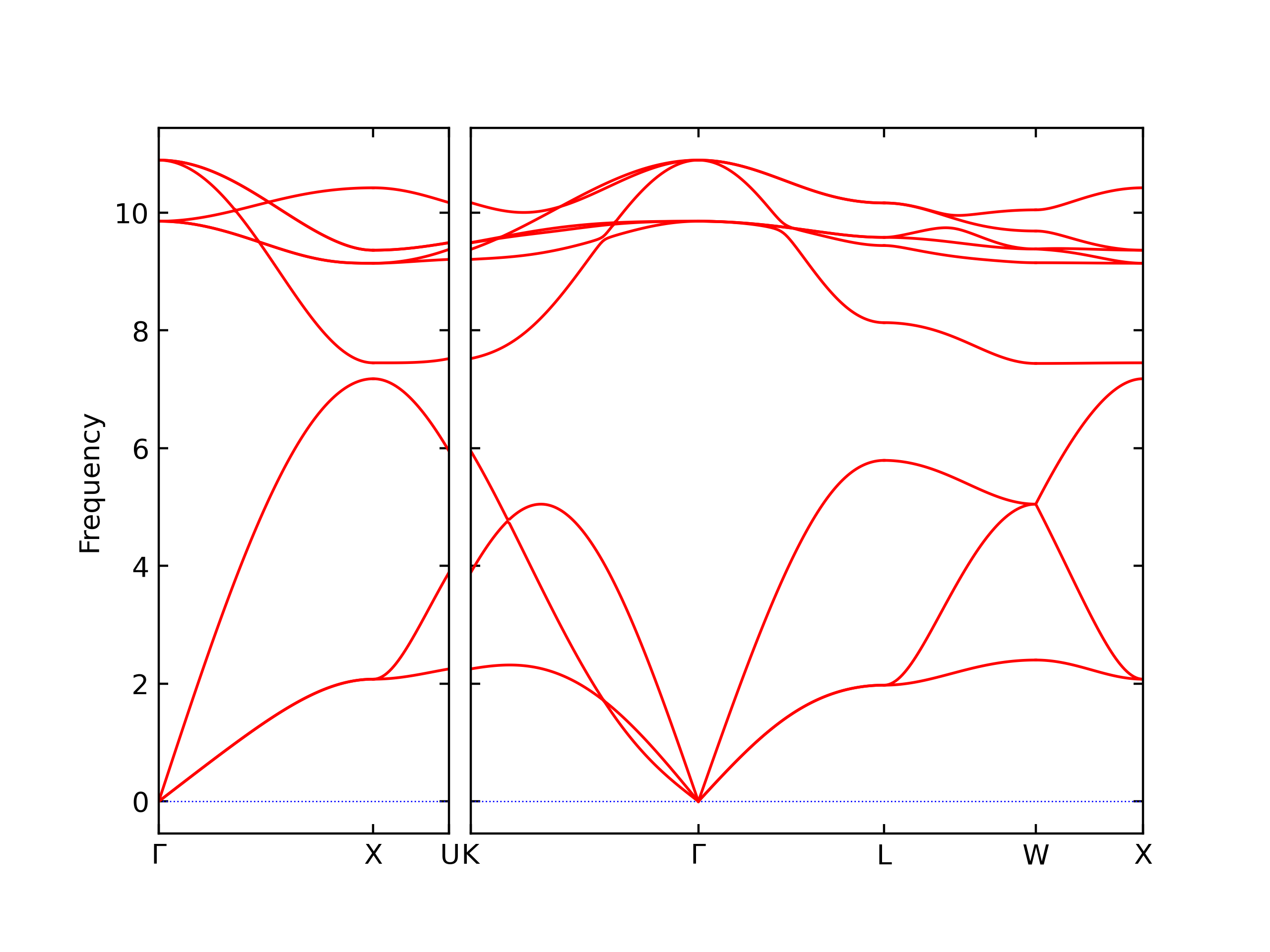
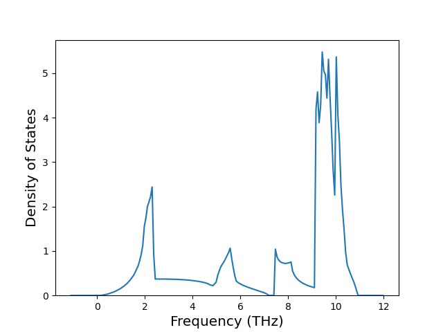
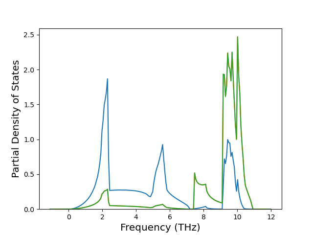
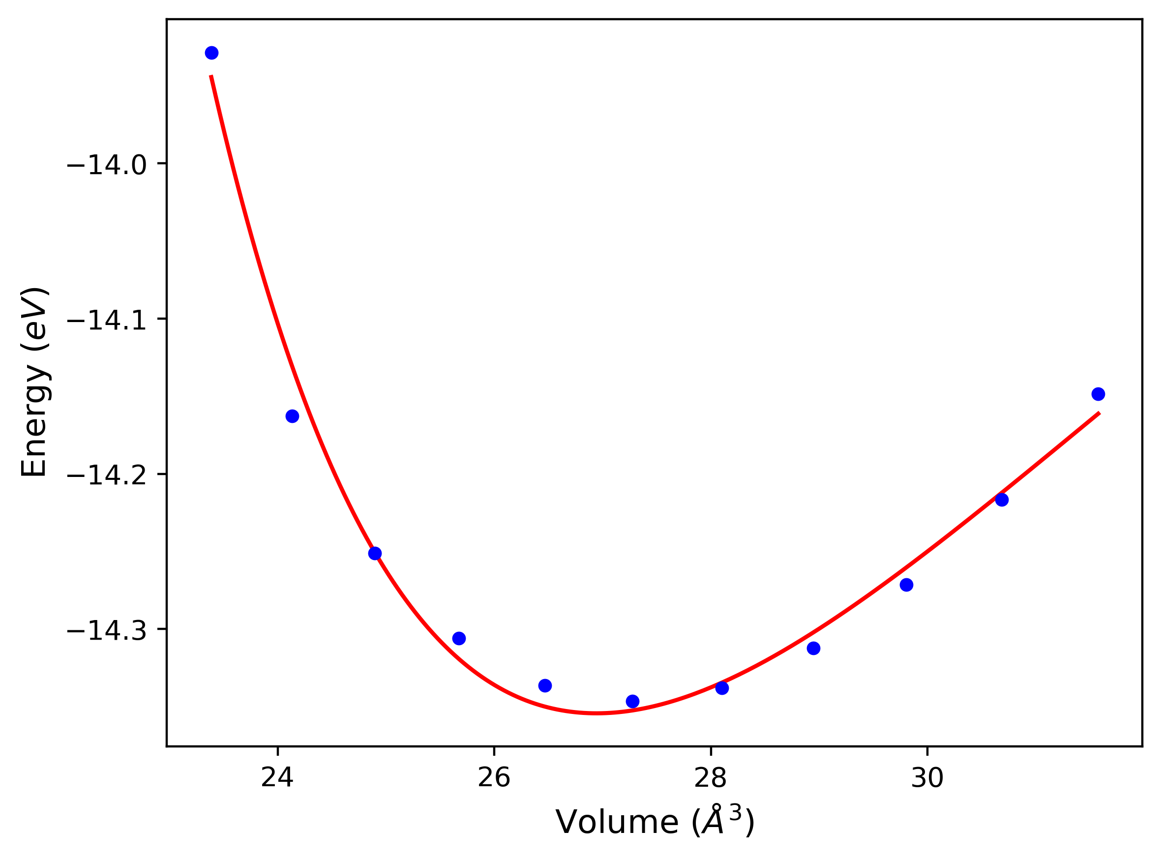
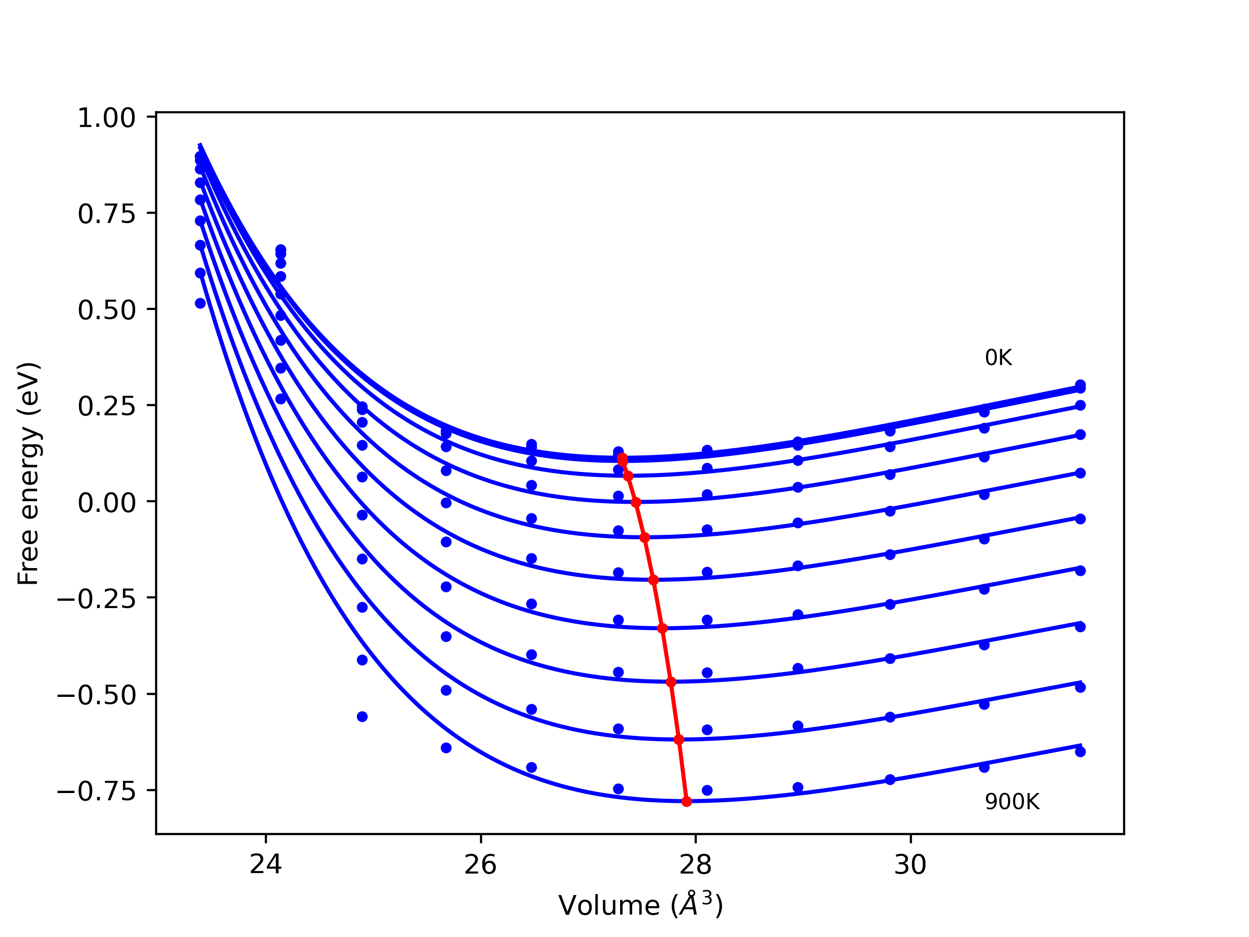
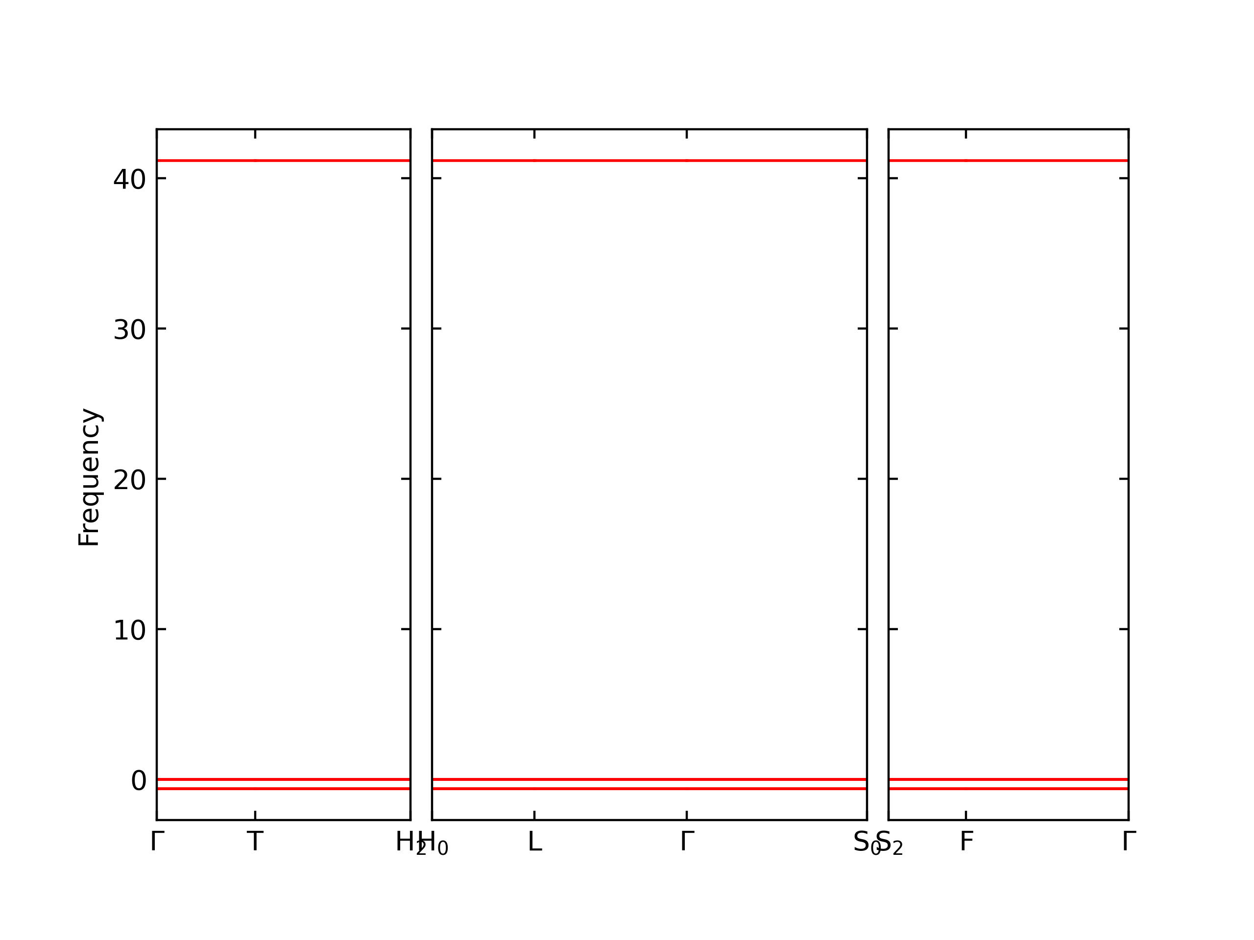


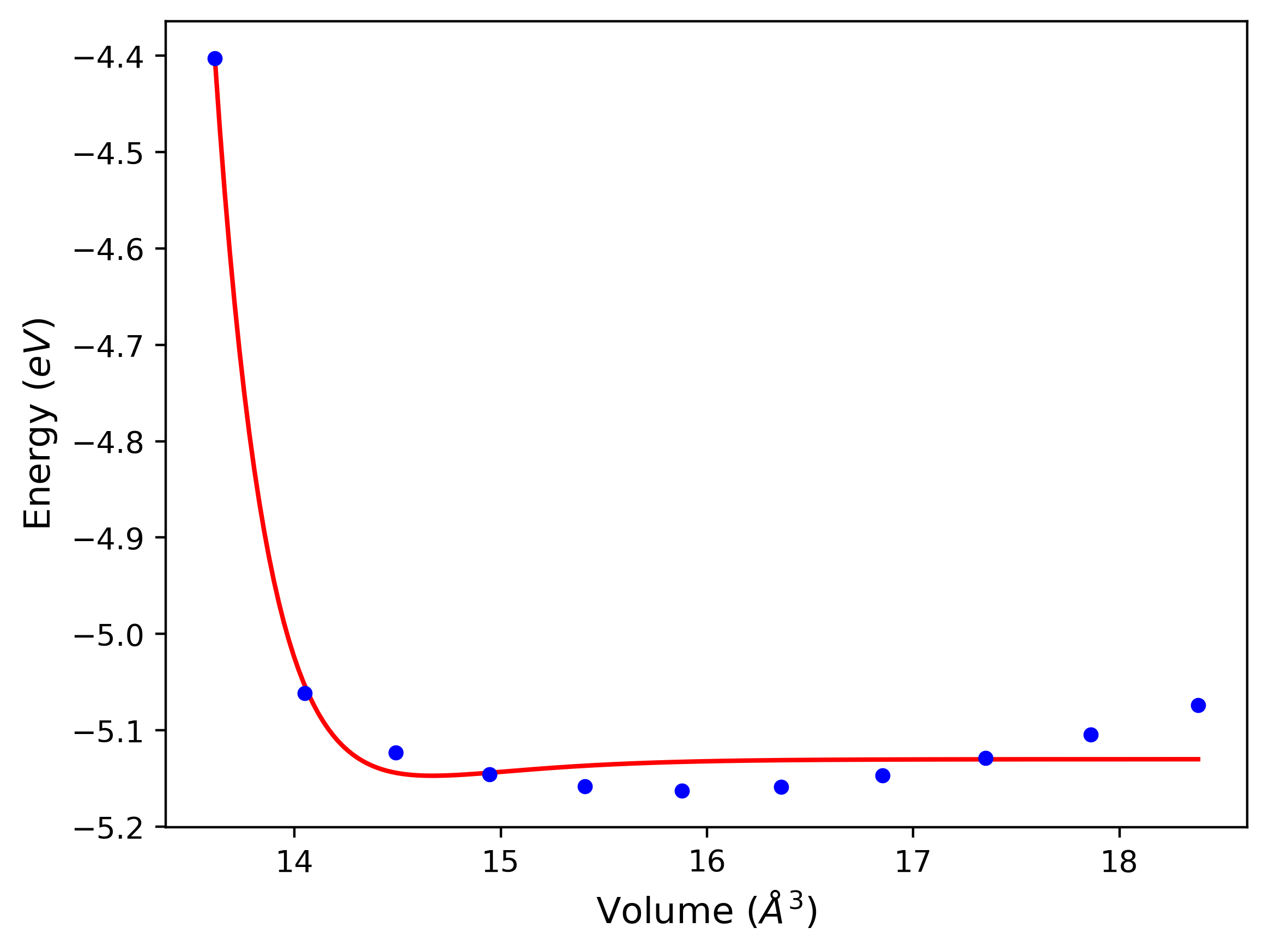
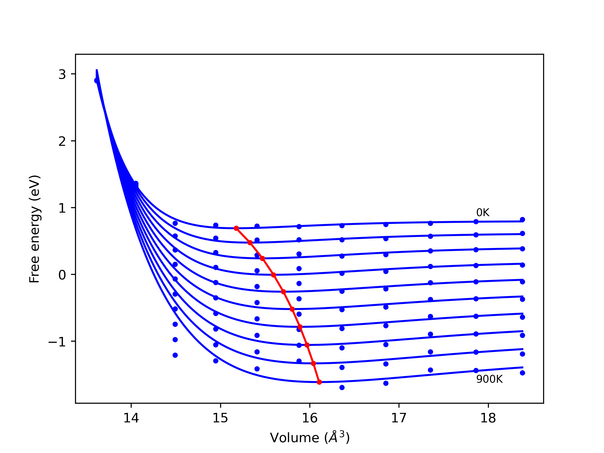
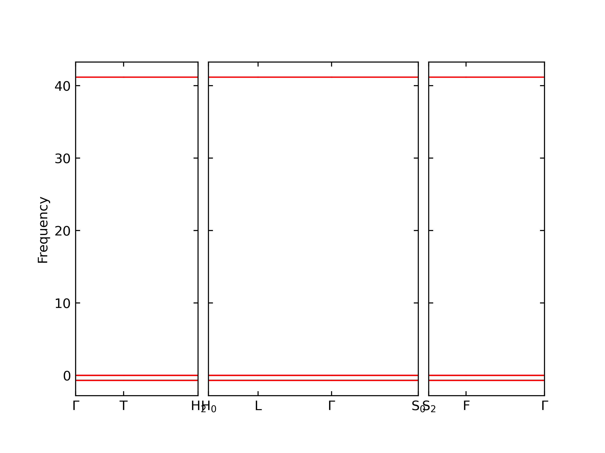

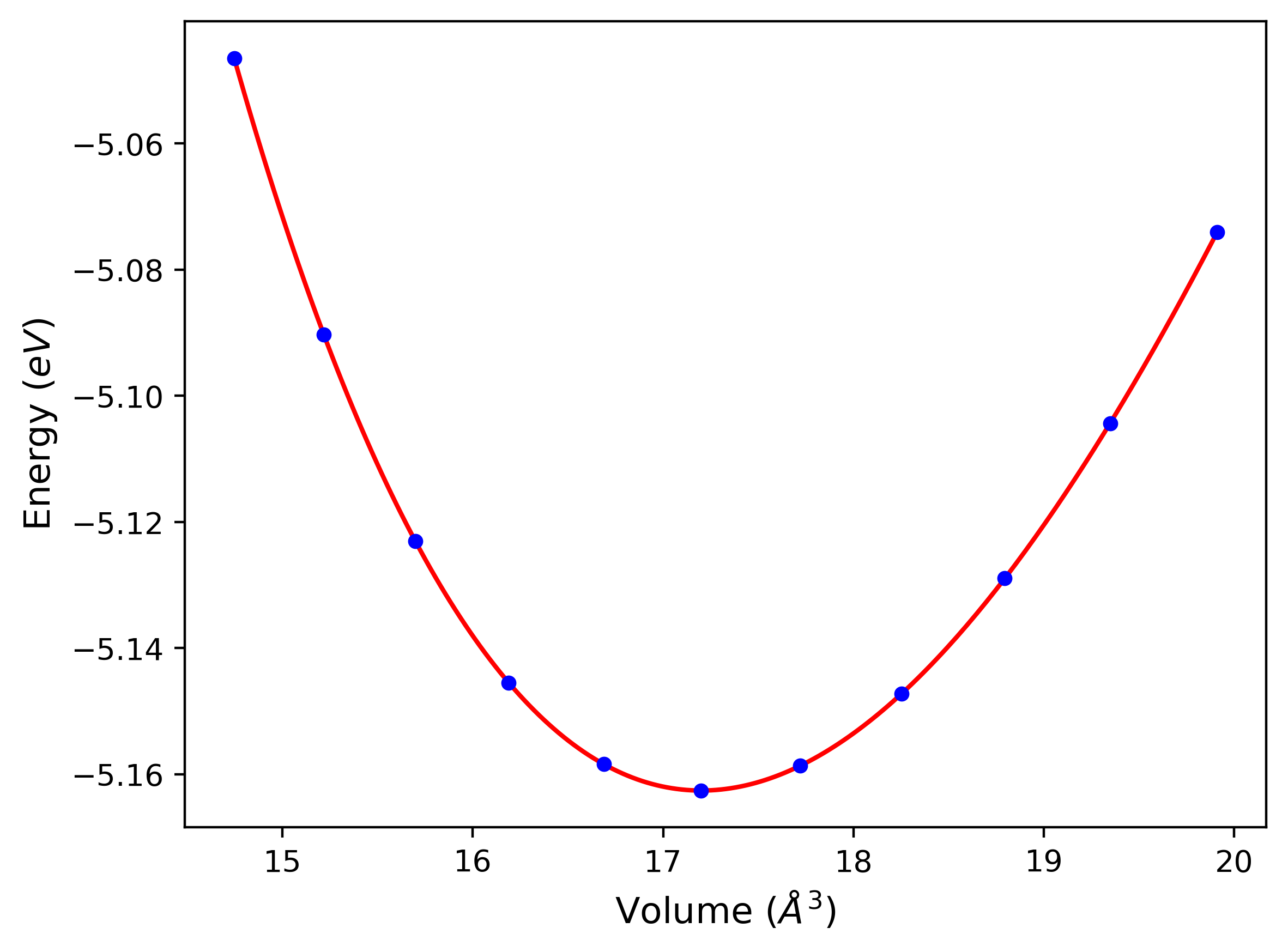
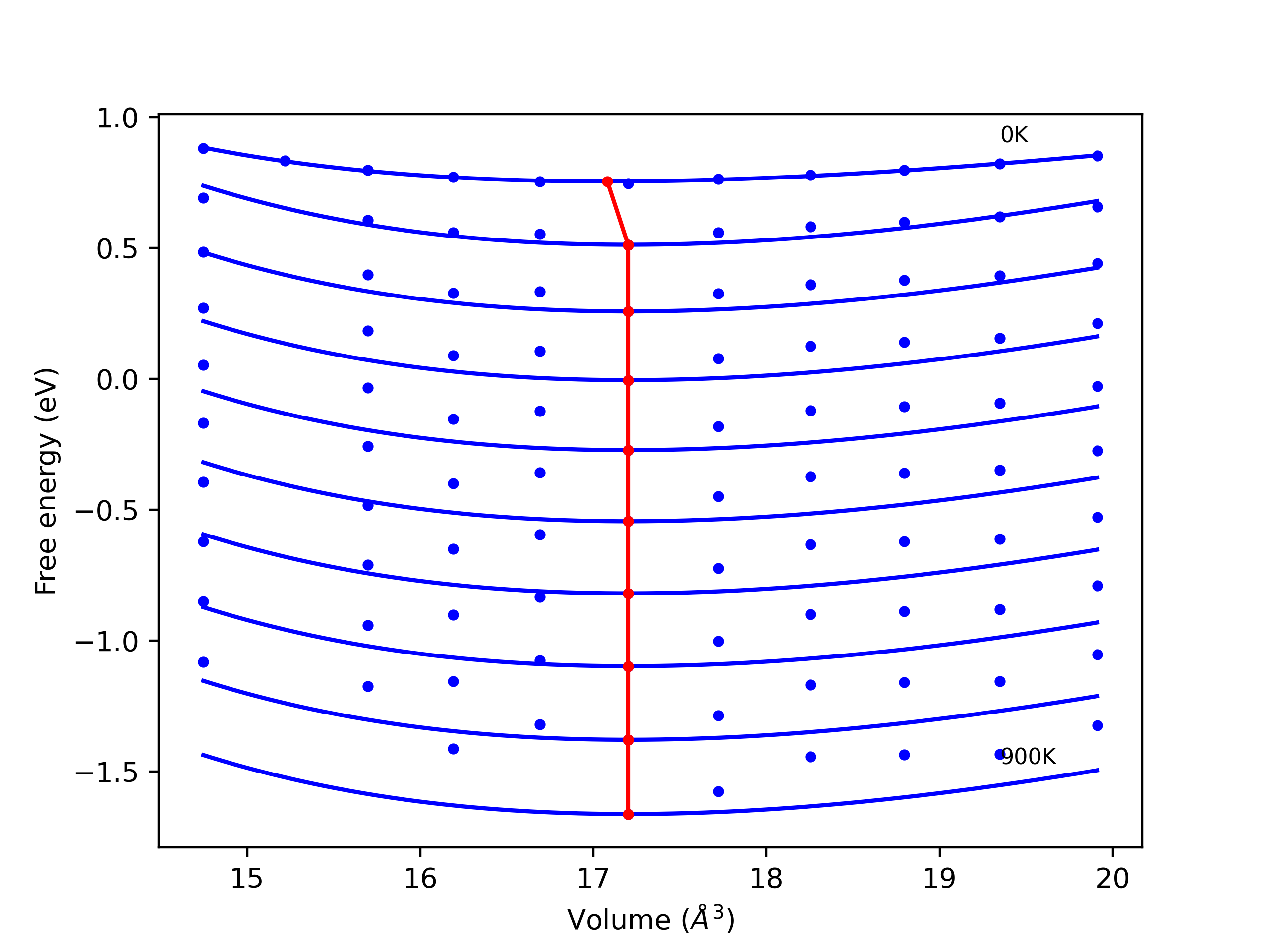
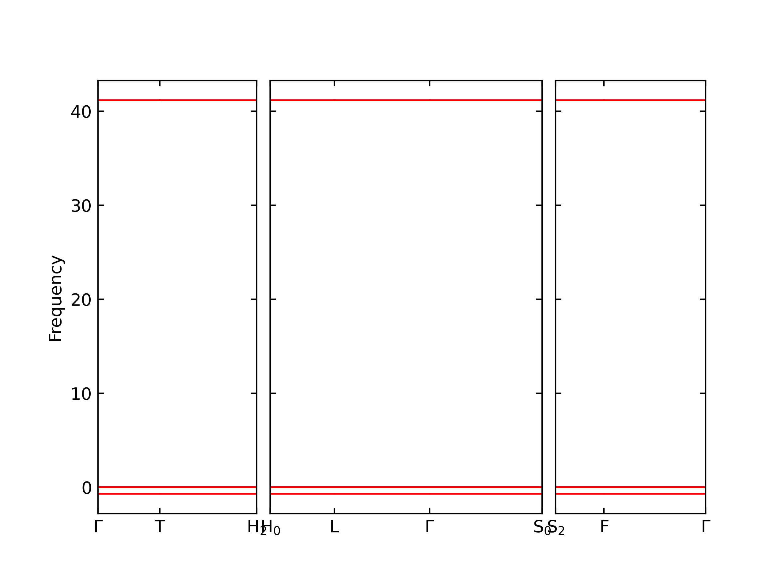
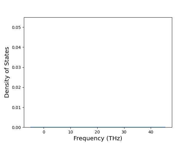

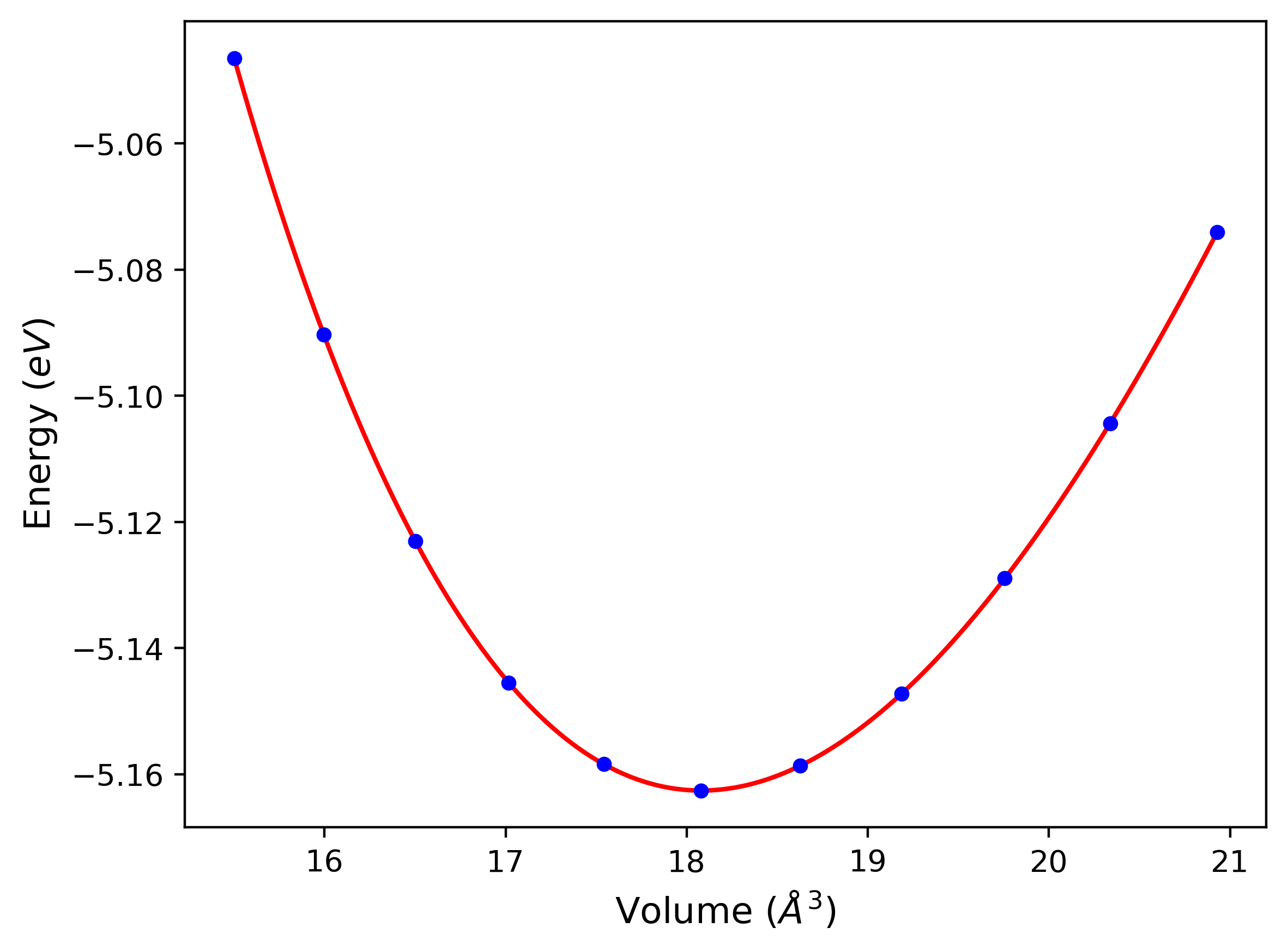
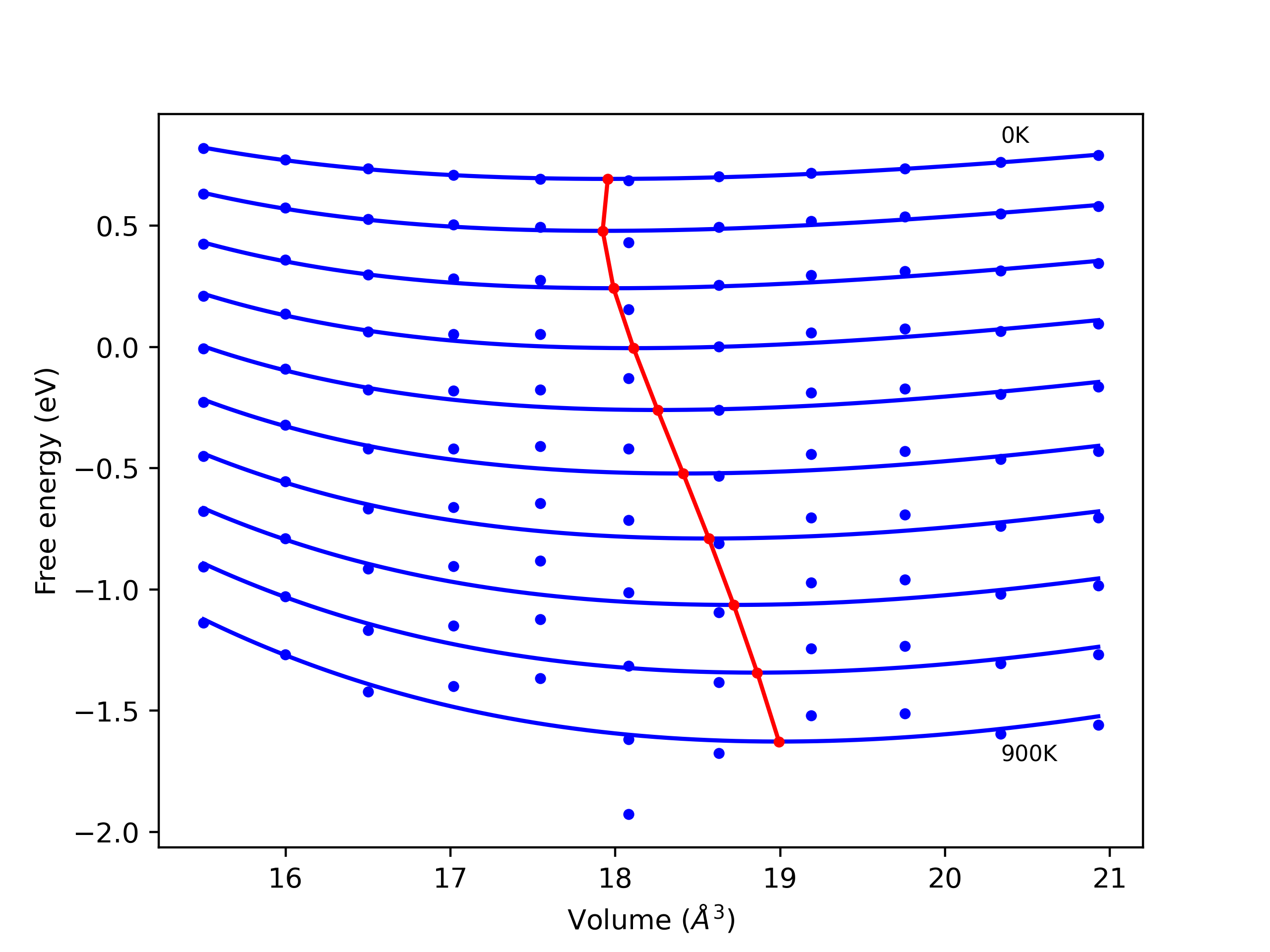
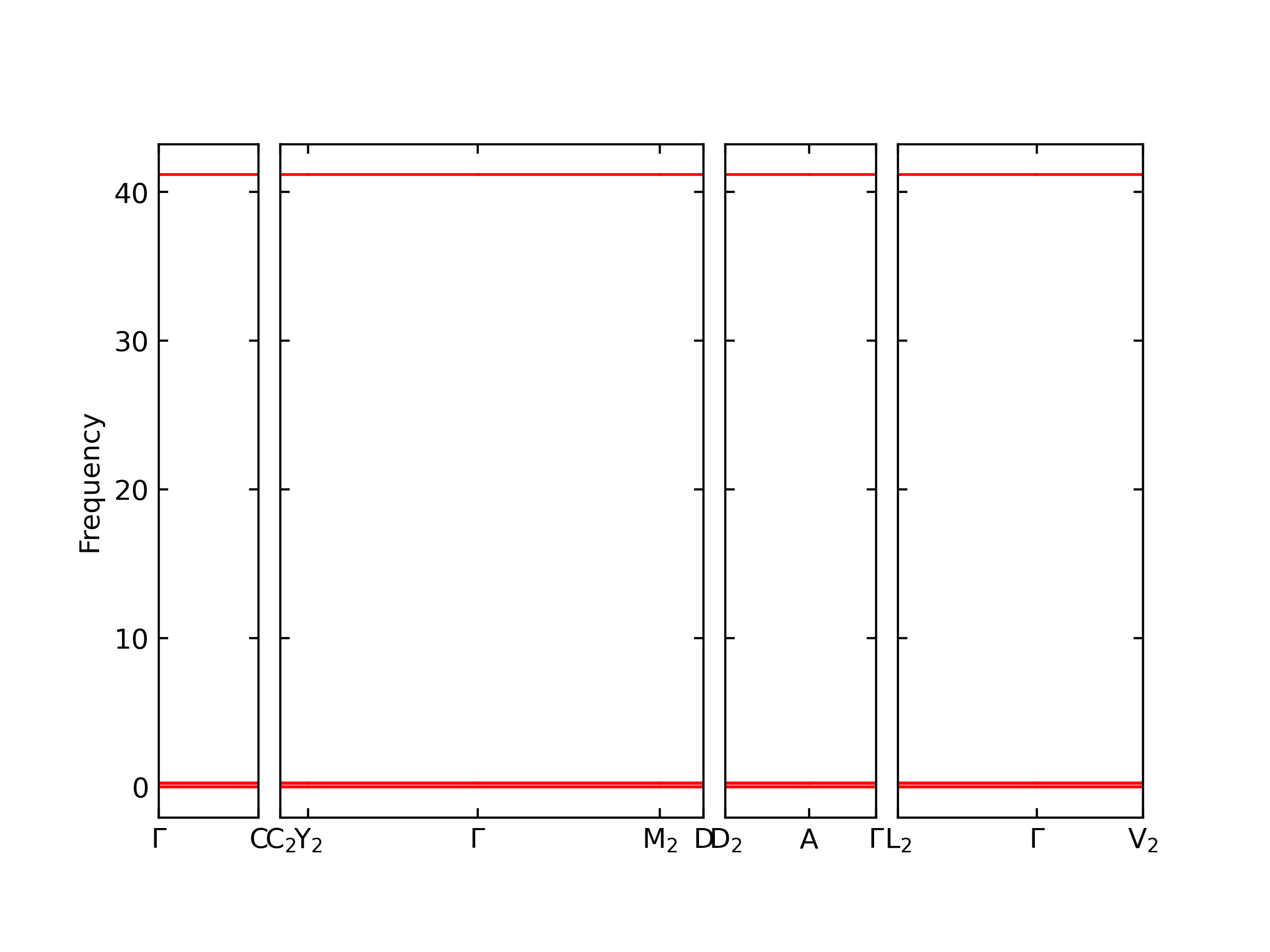


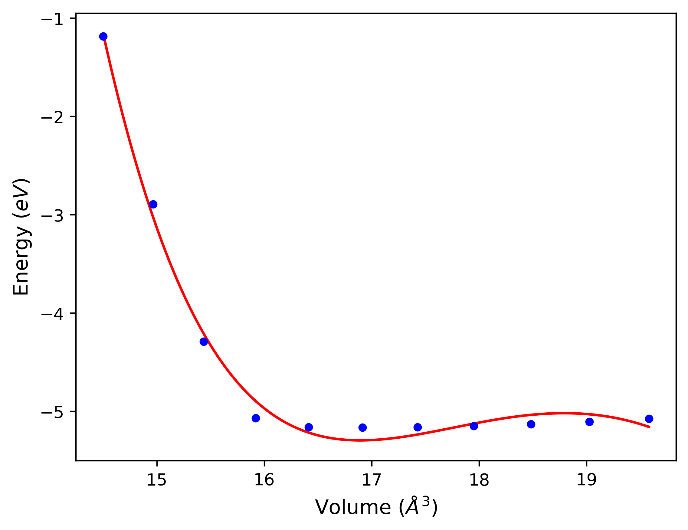
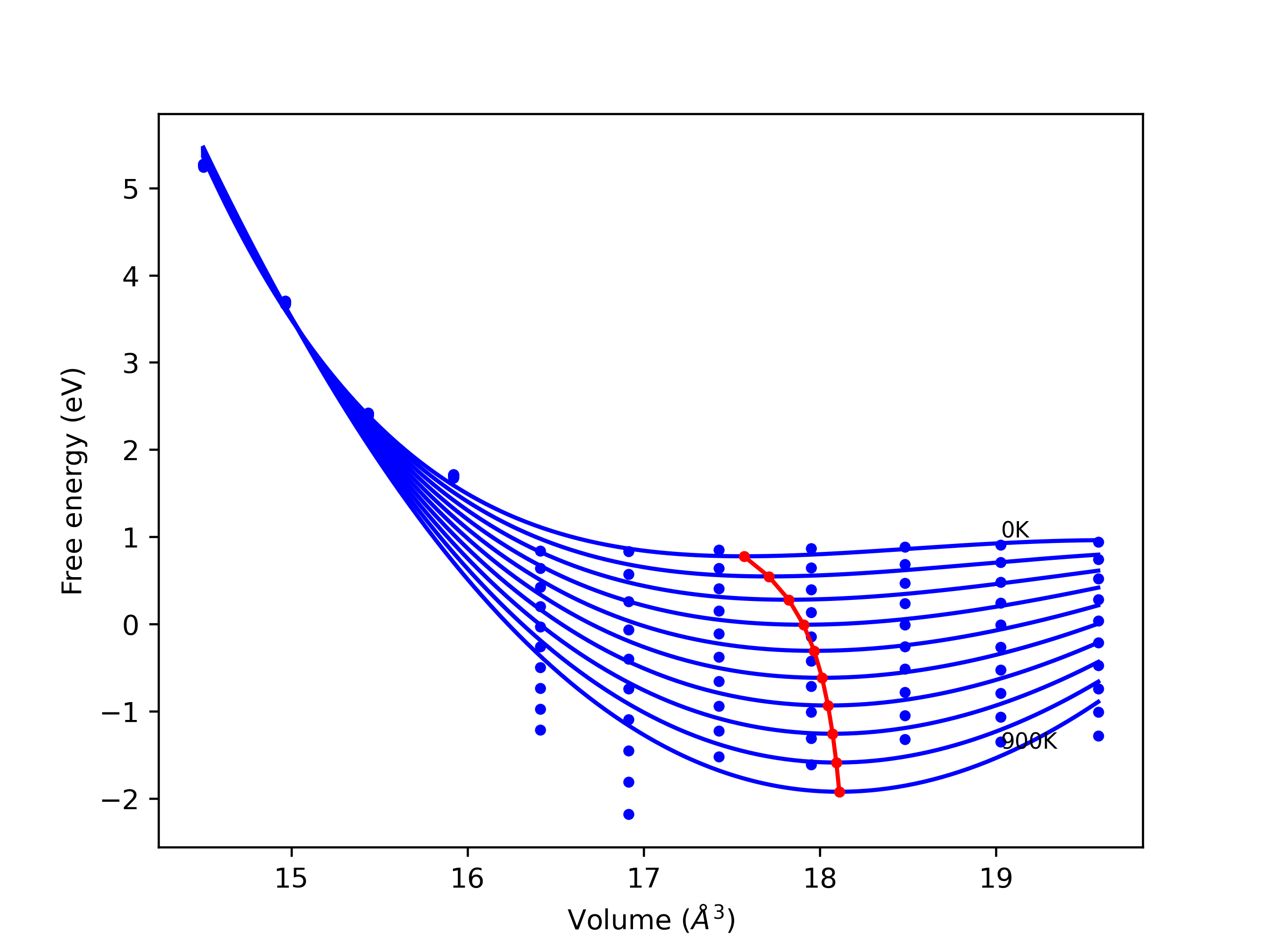
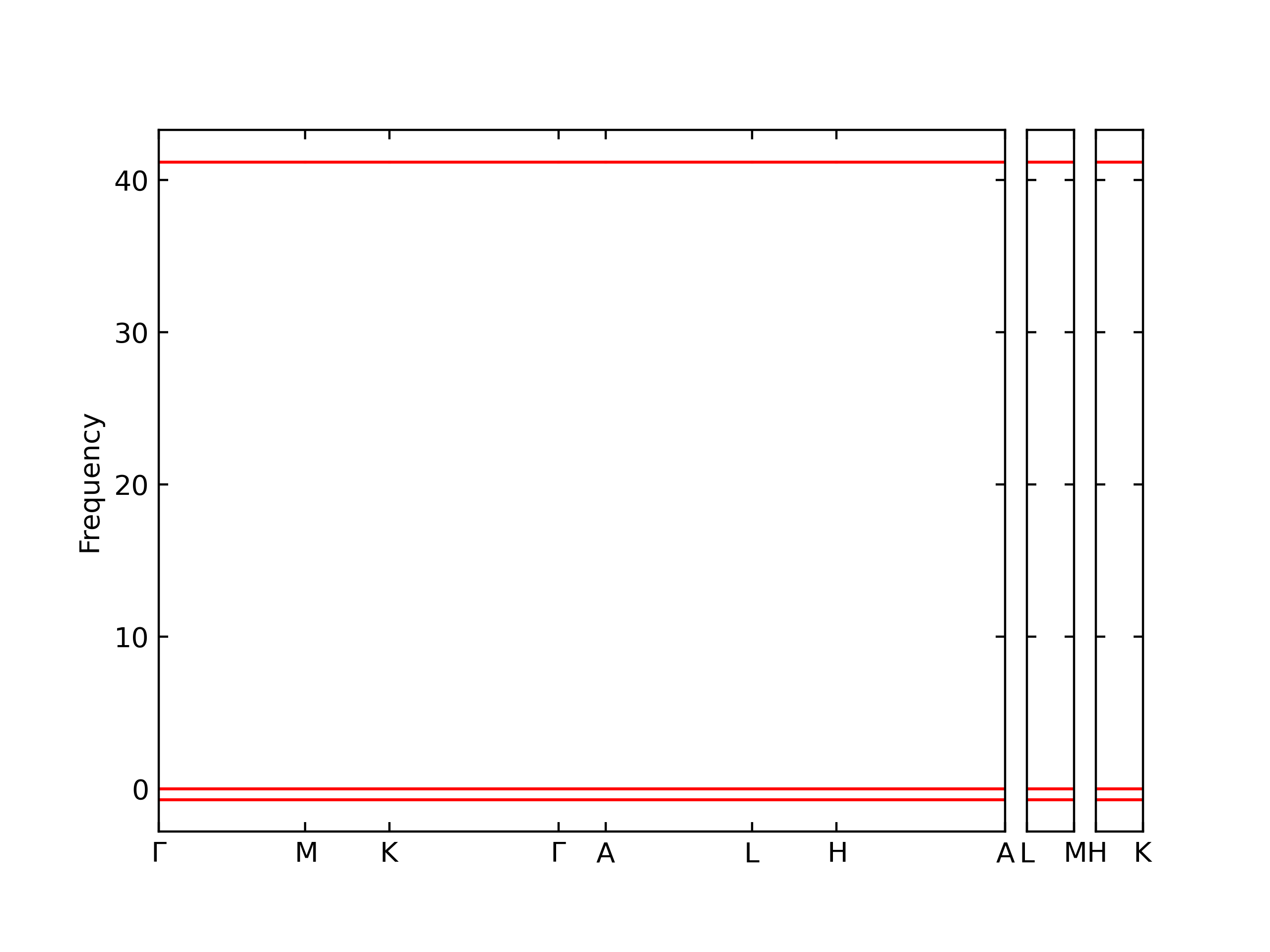


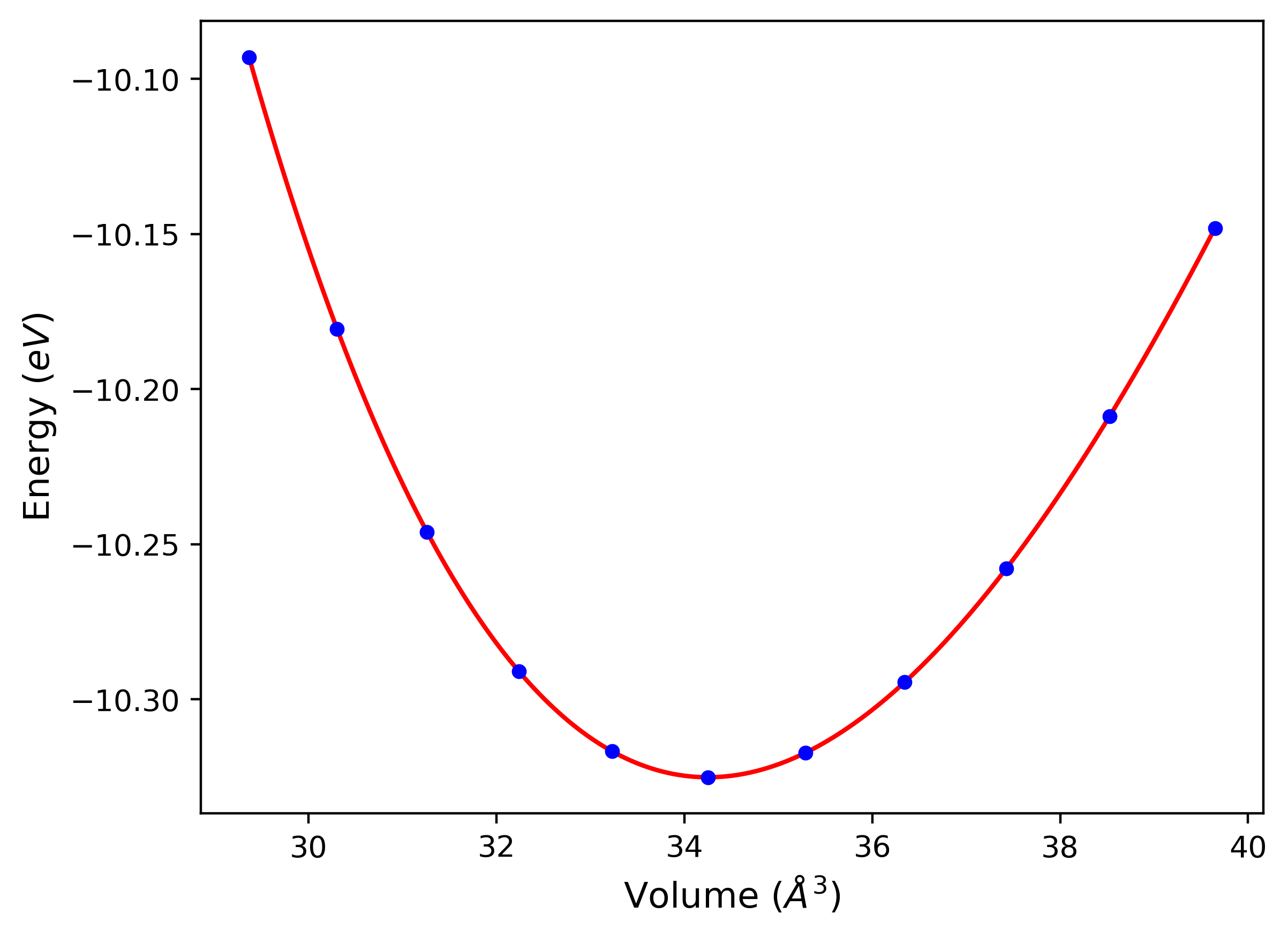
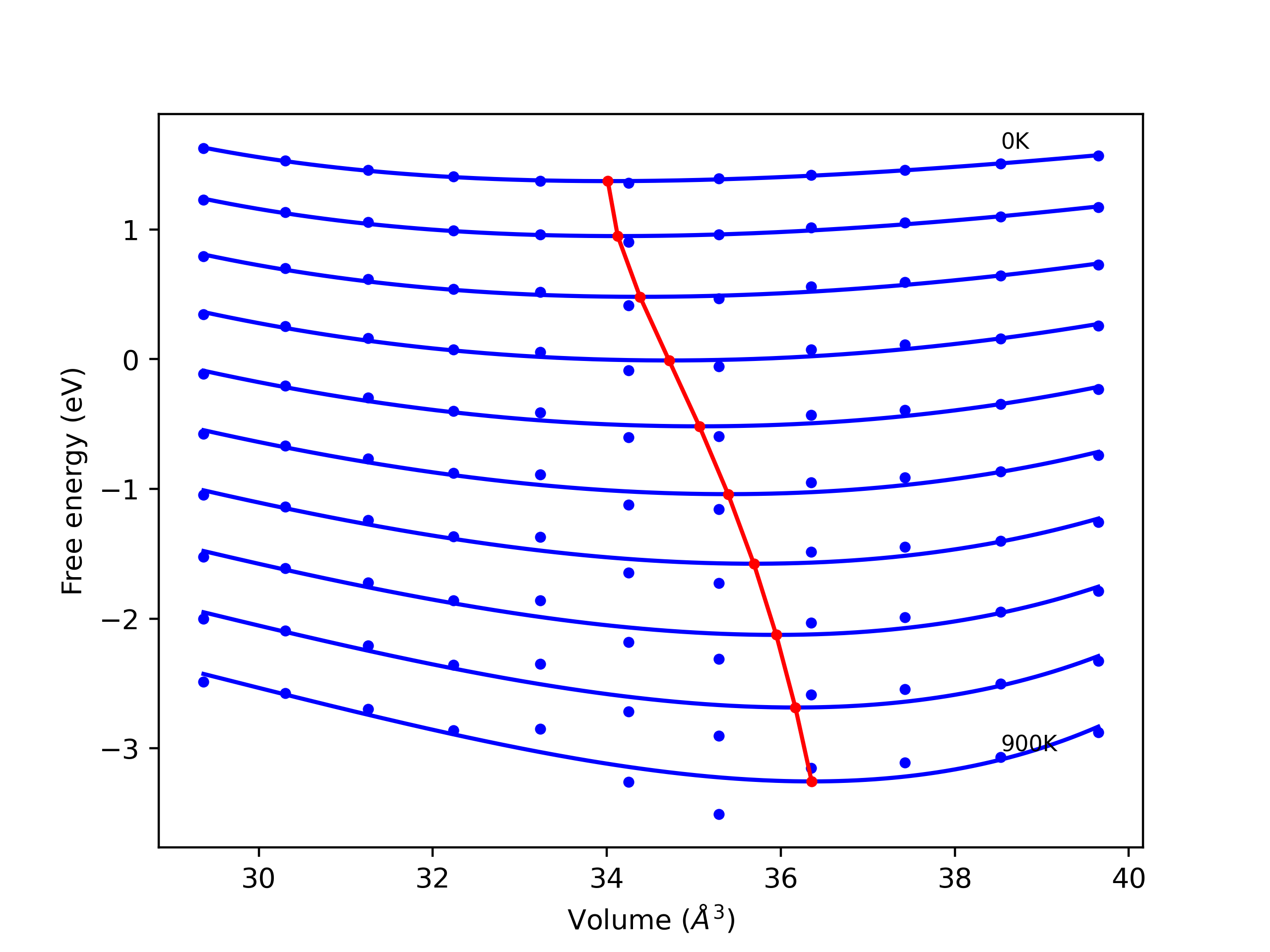
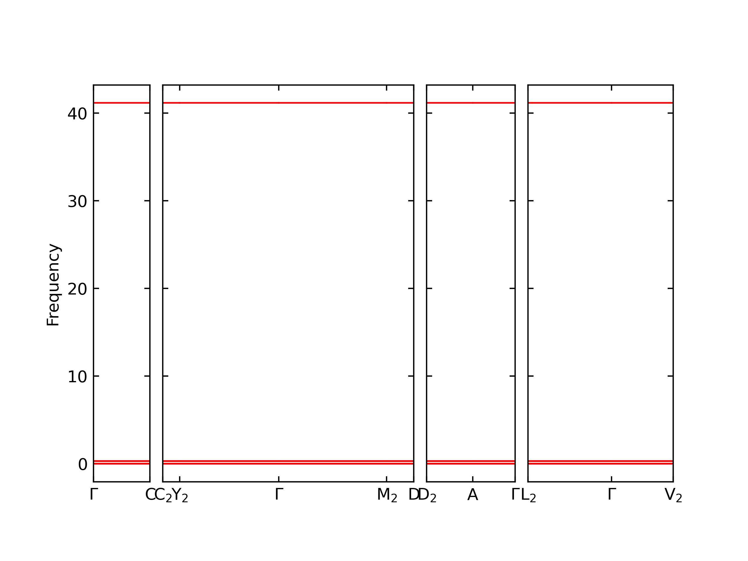


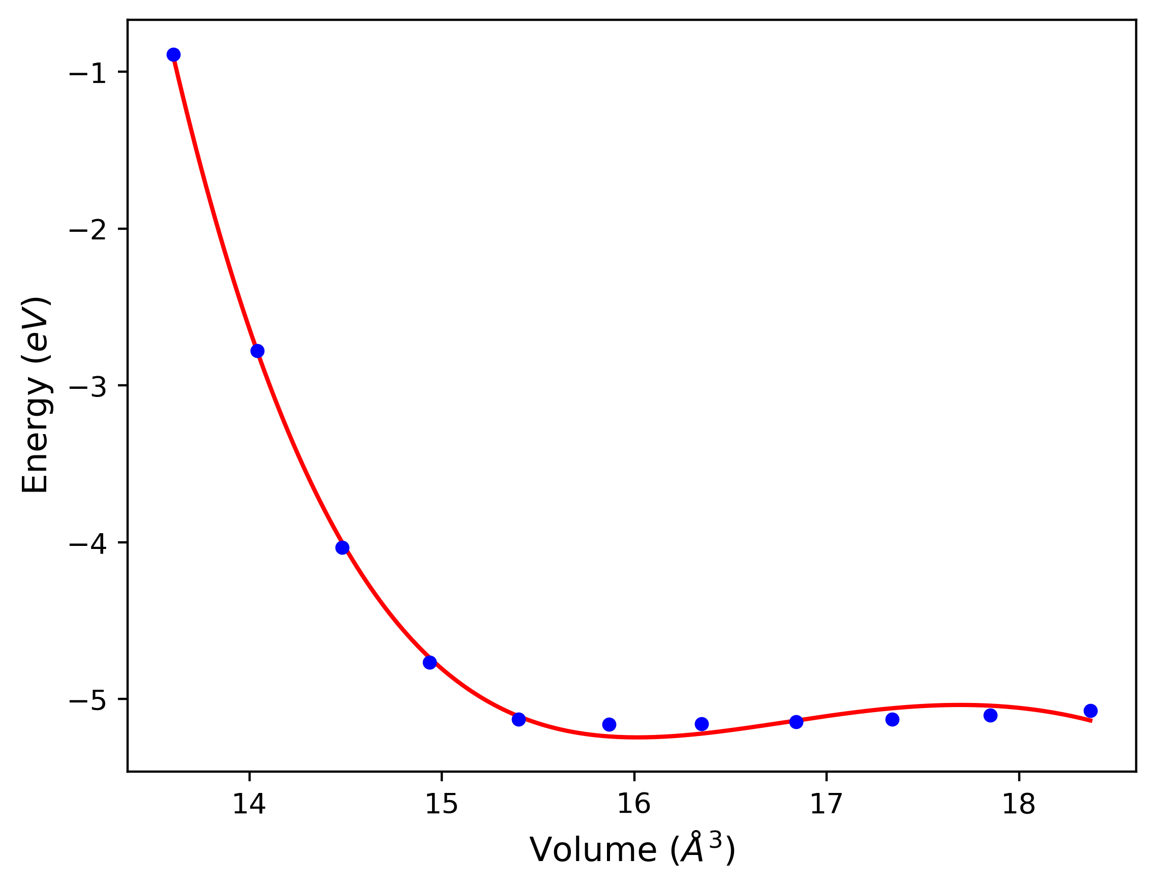
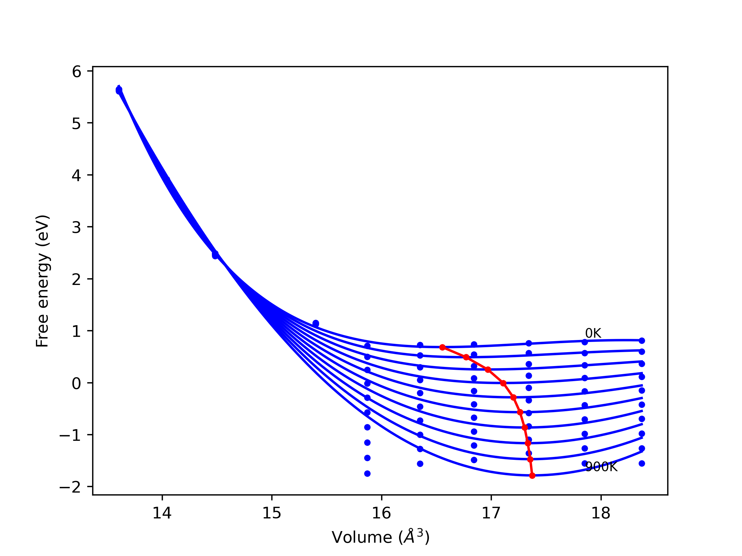
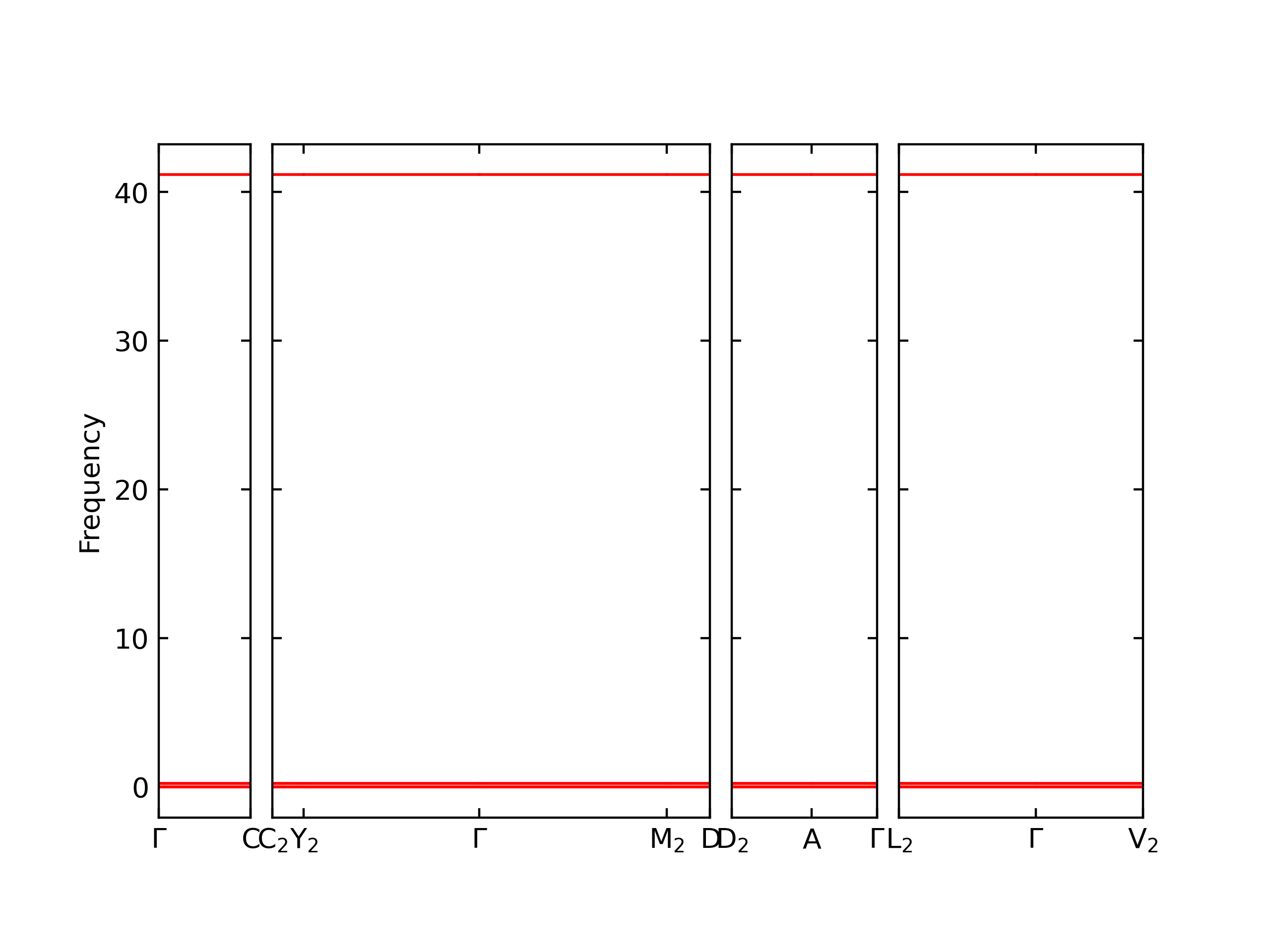


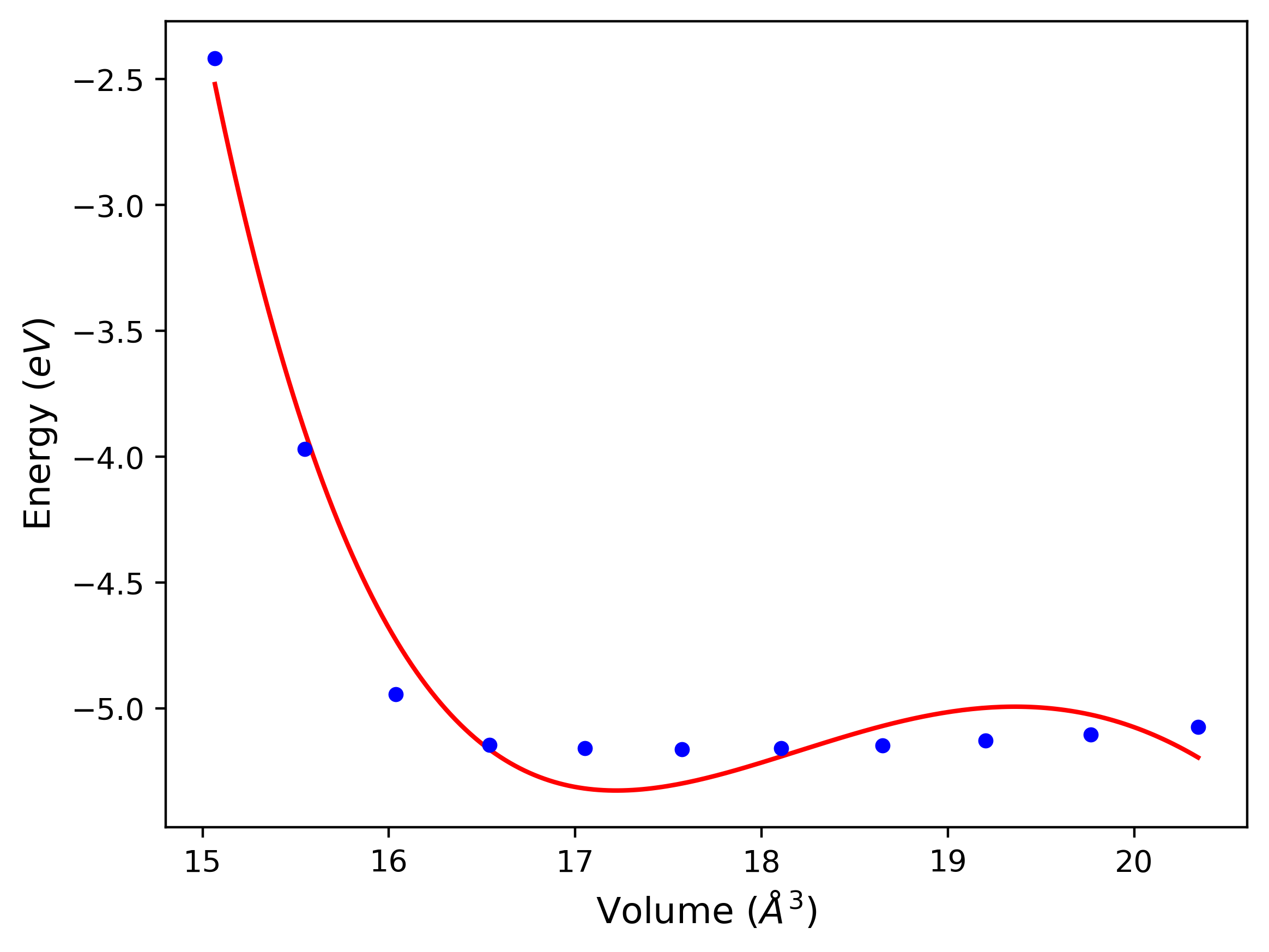
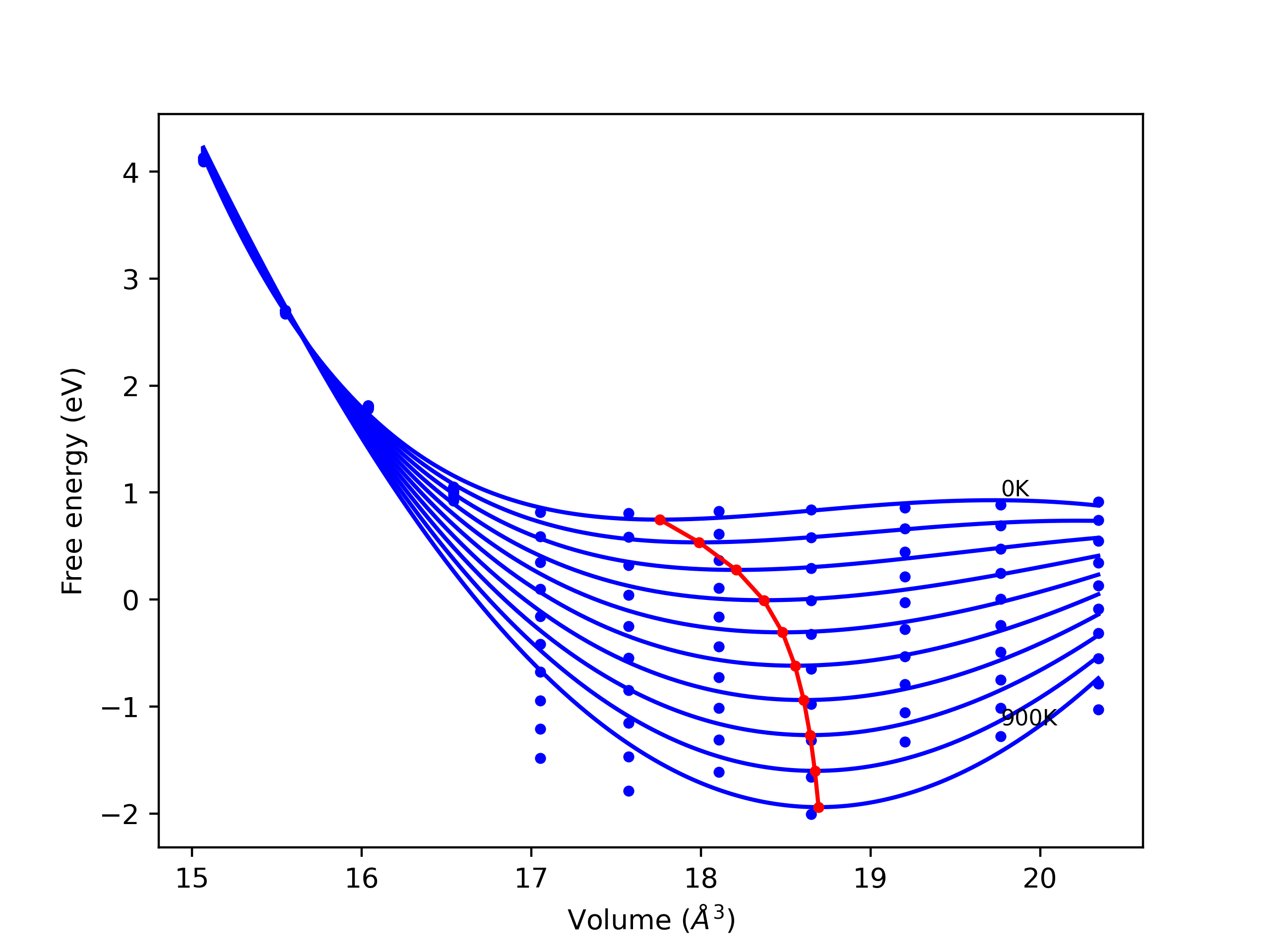
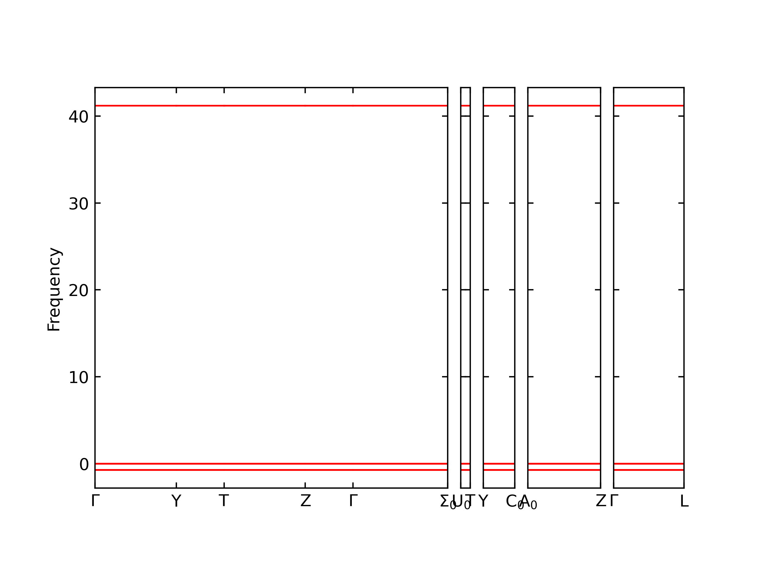


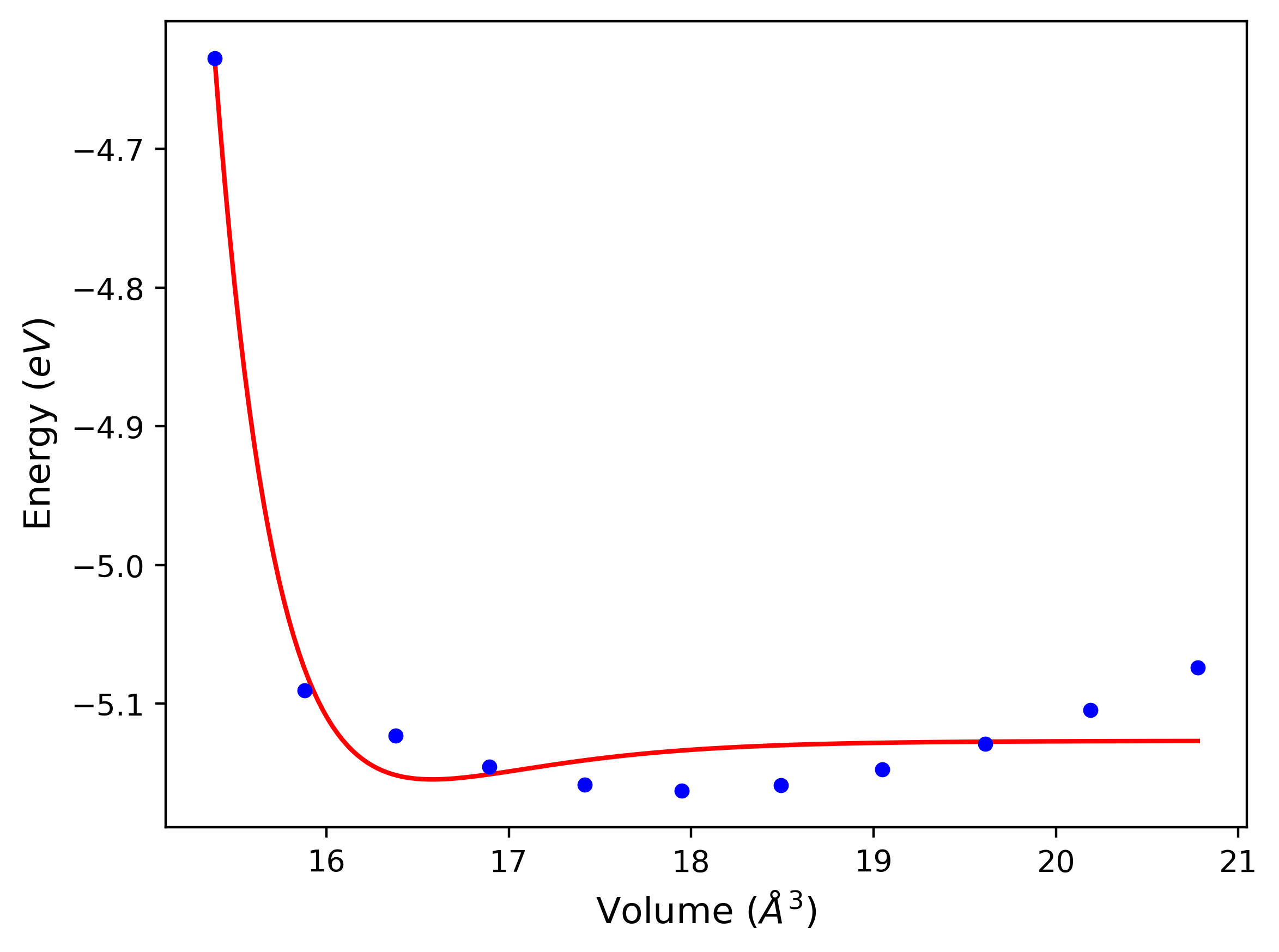
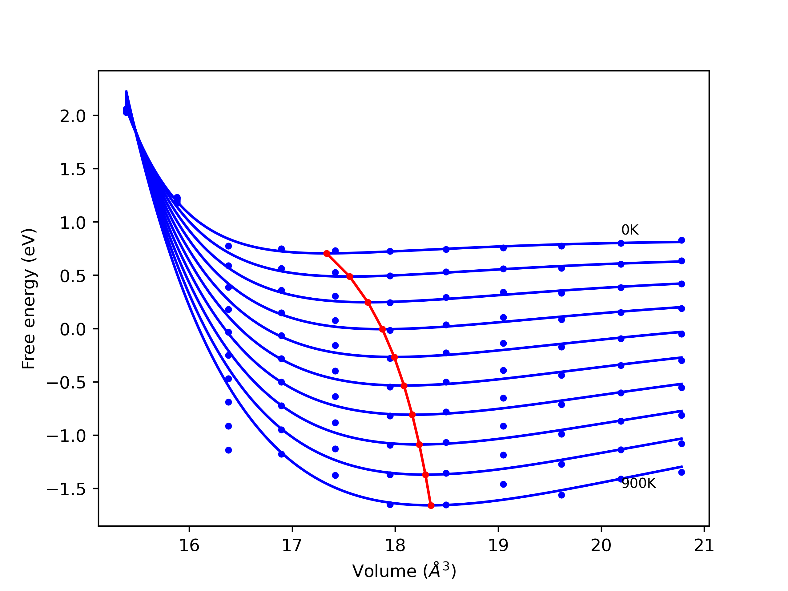
Thermodynamic Predictions
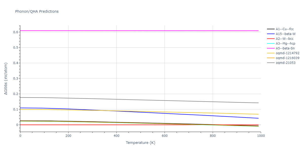
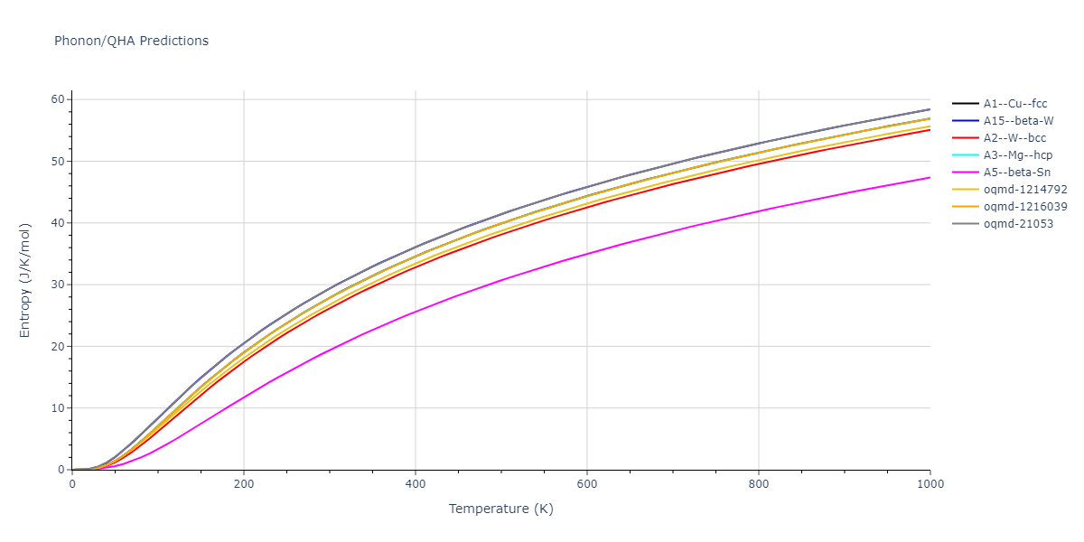
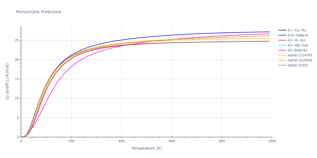
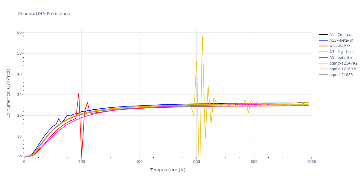
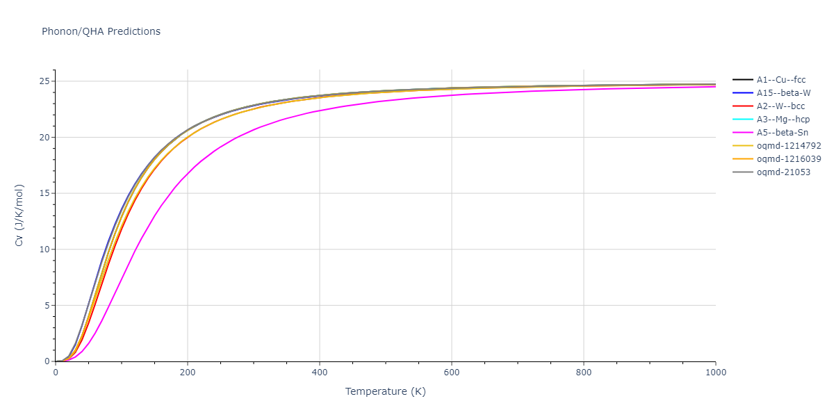
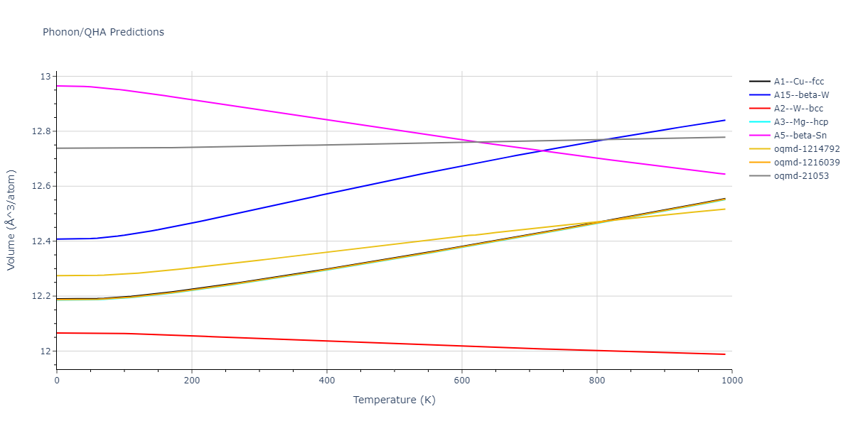
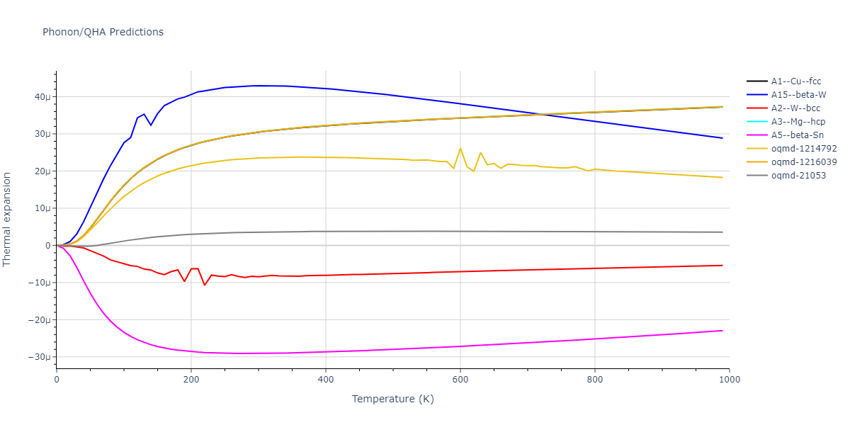
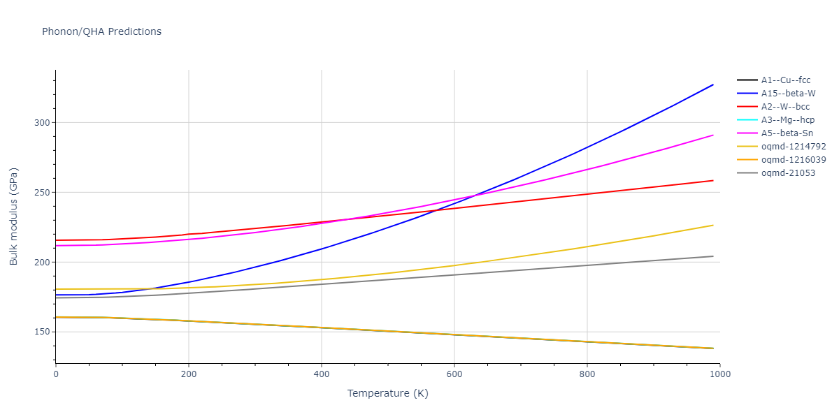
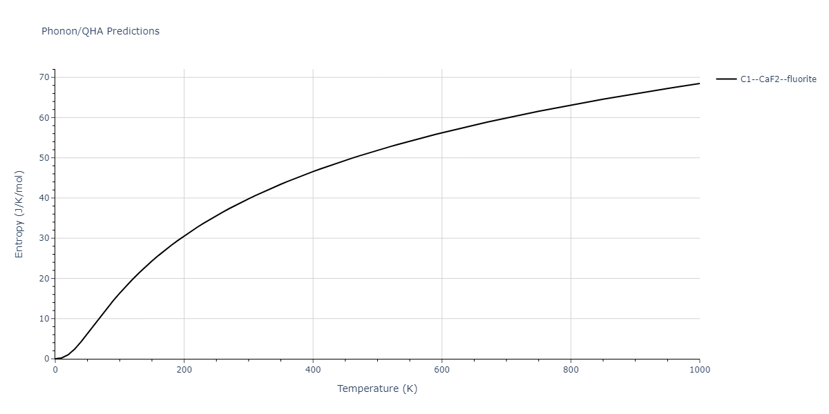

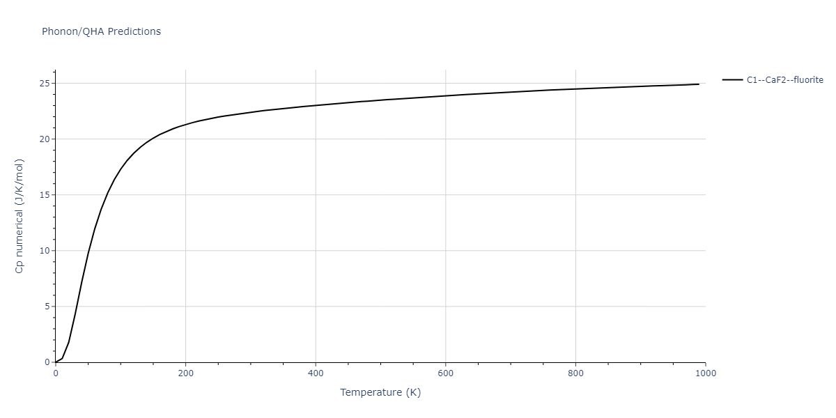
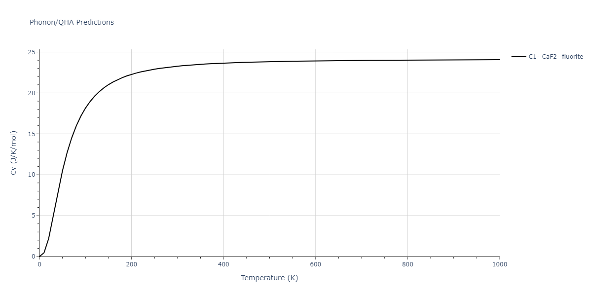
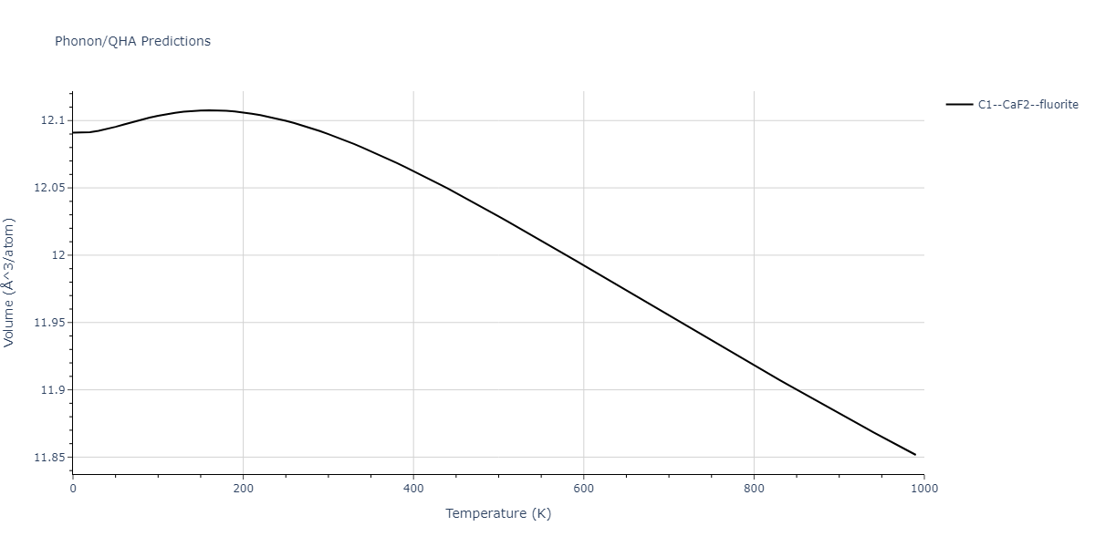
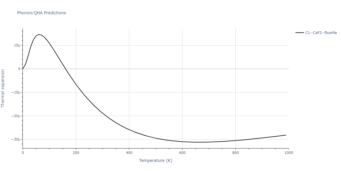
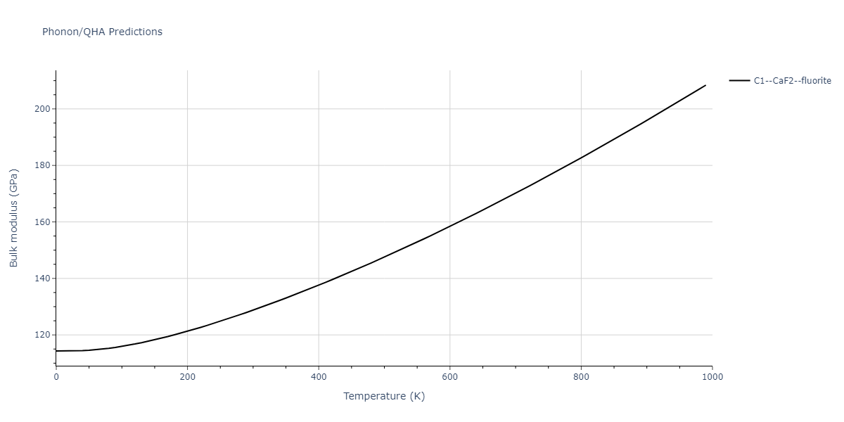
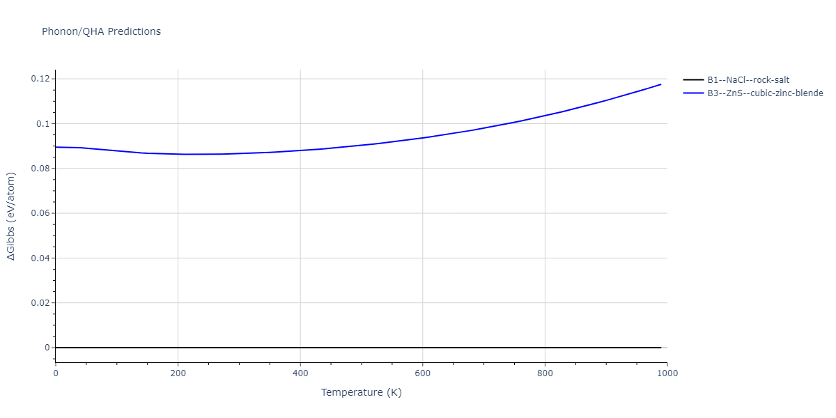
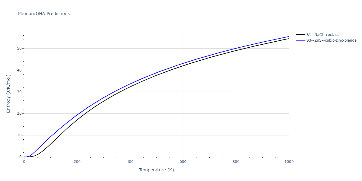
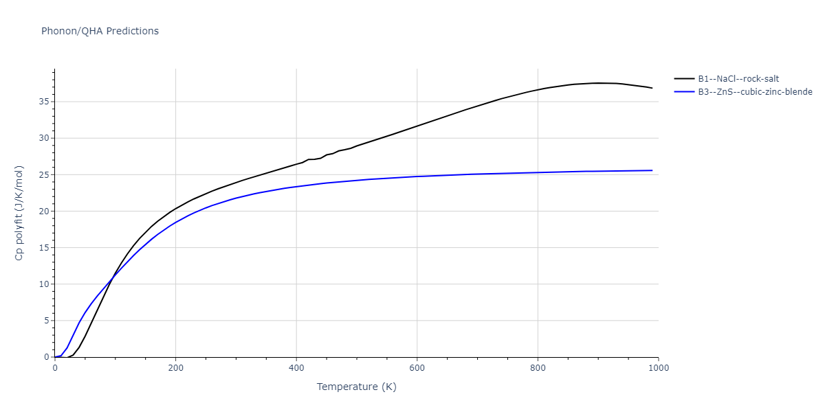
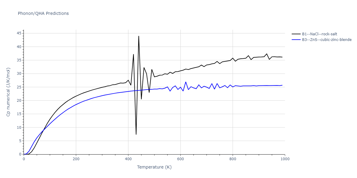
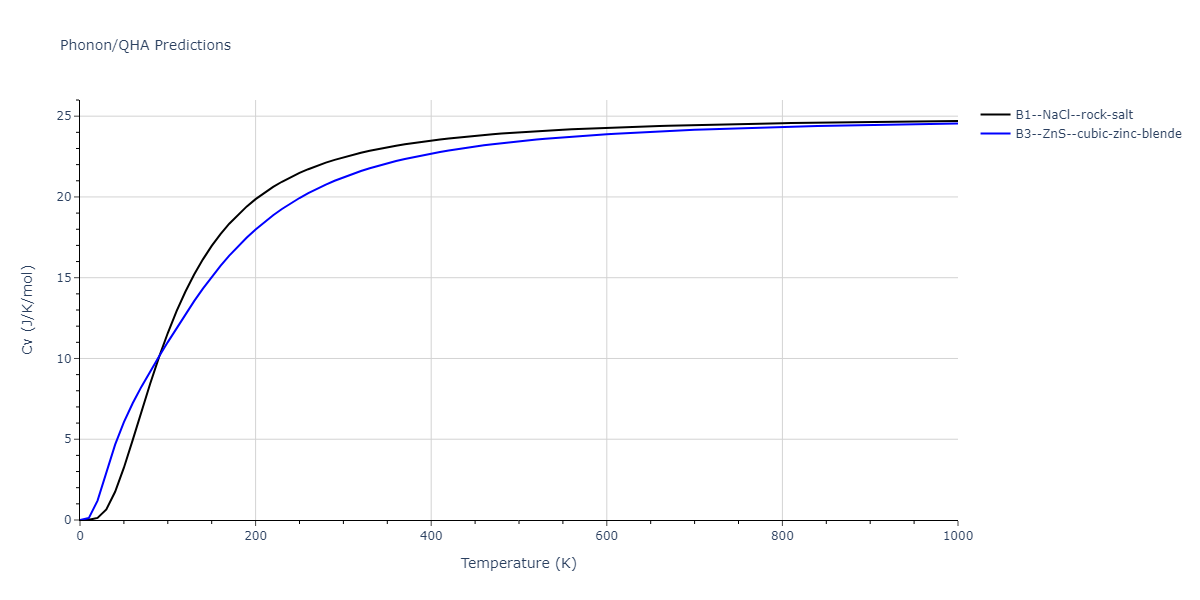
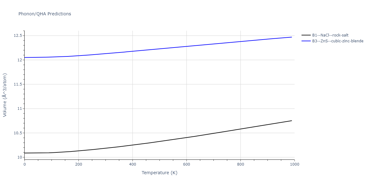
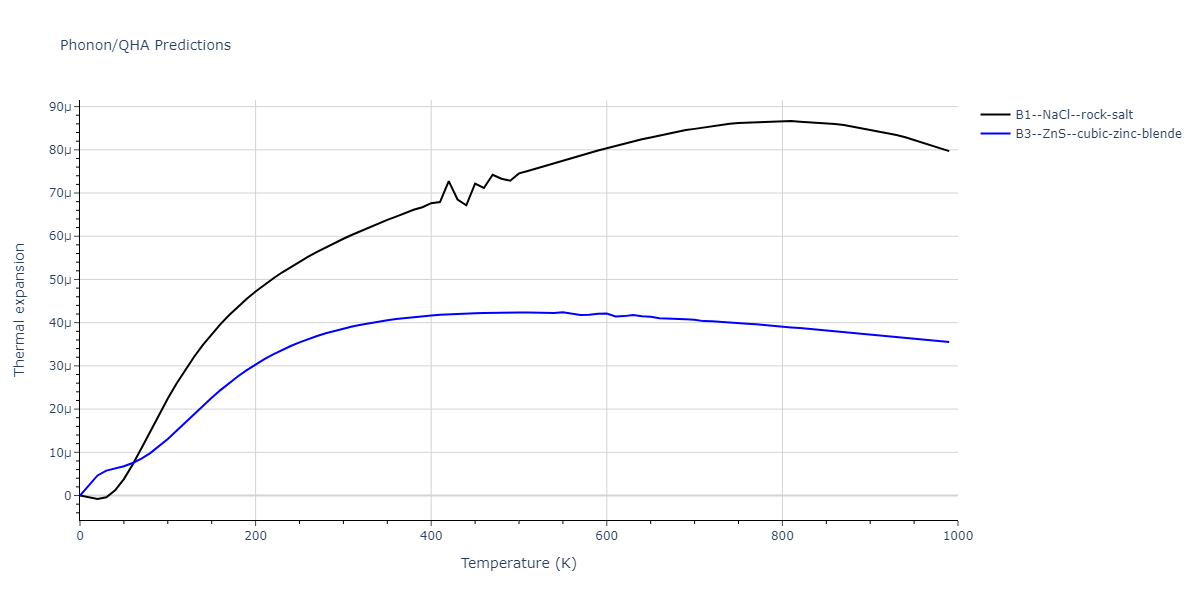
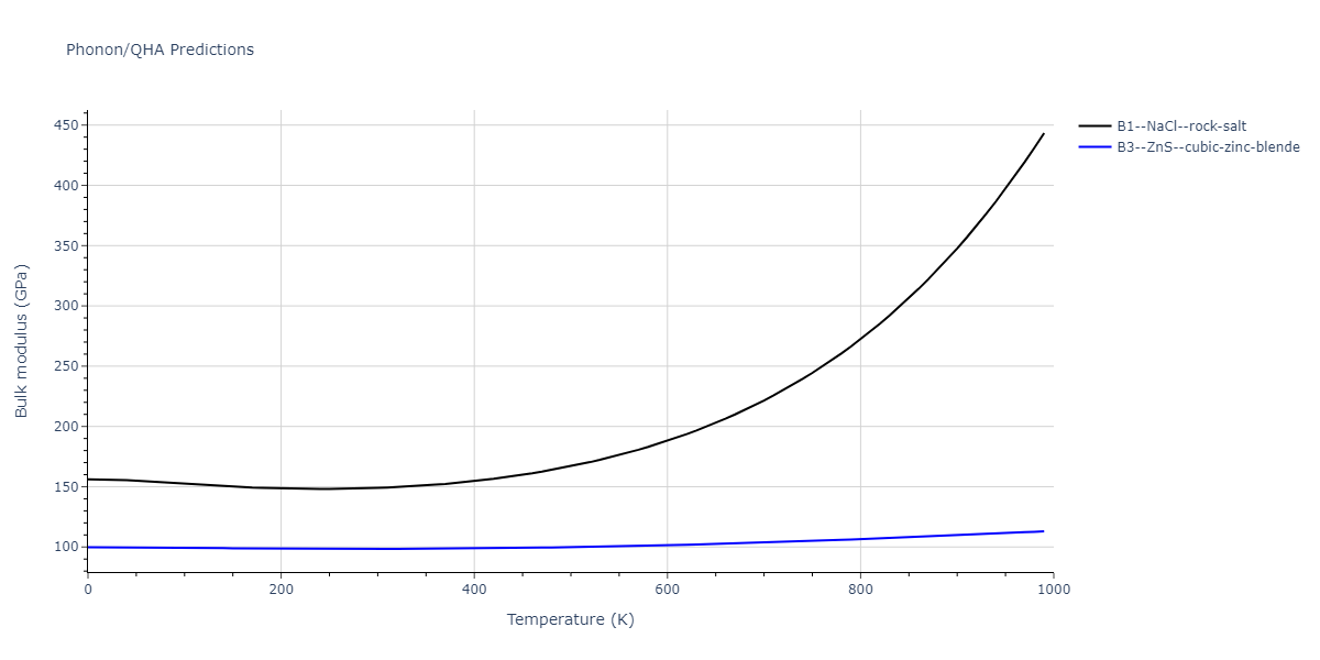

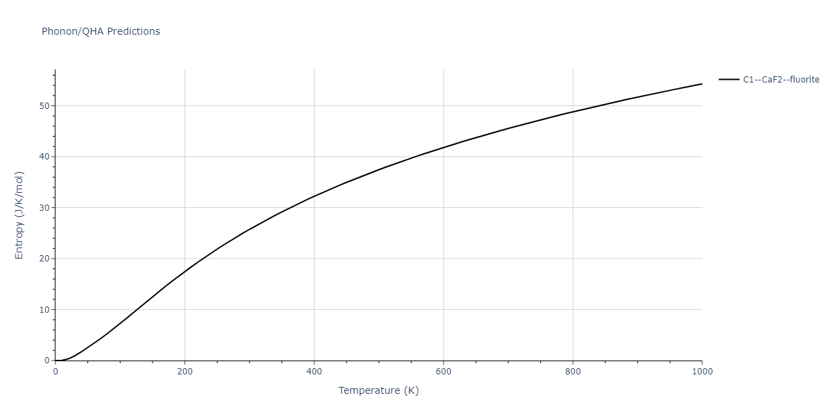
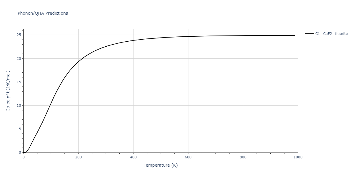
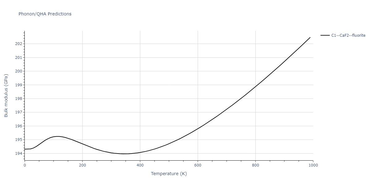
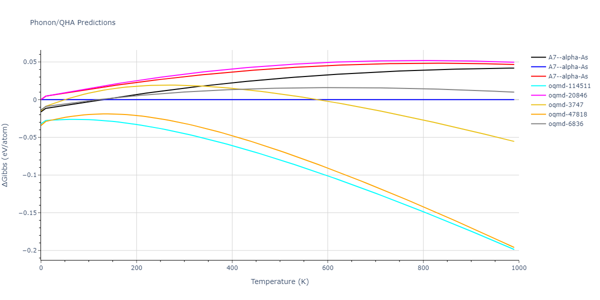
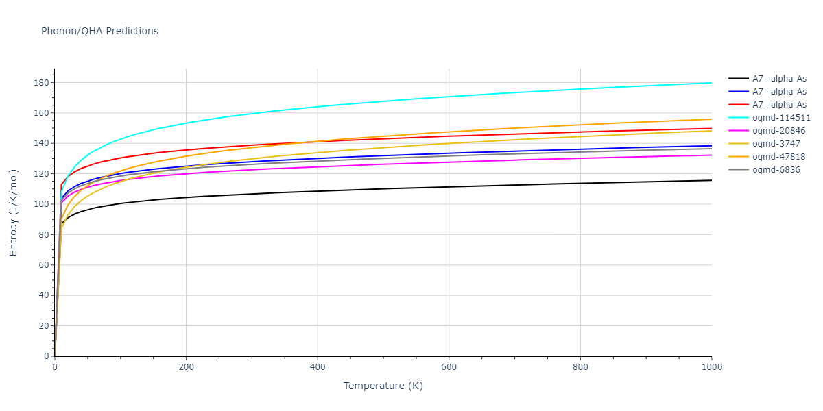
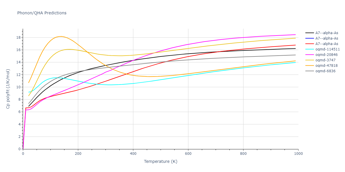
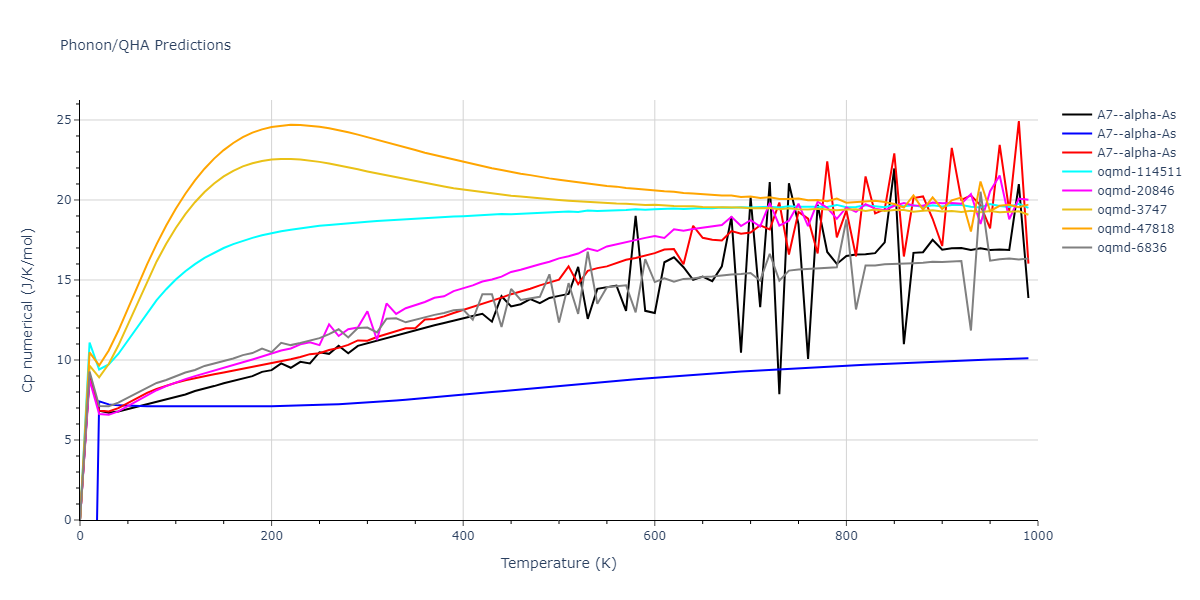
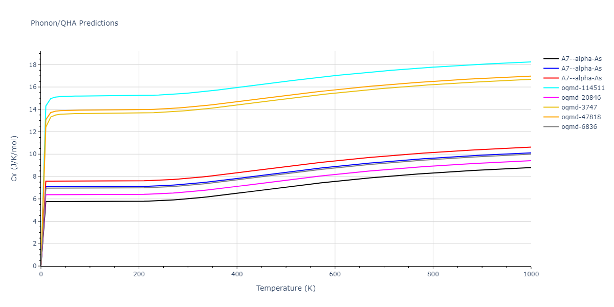
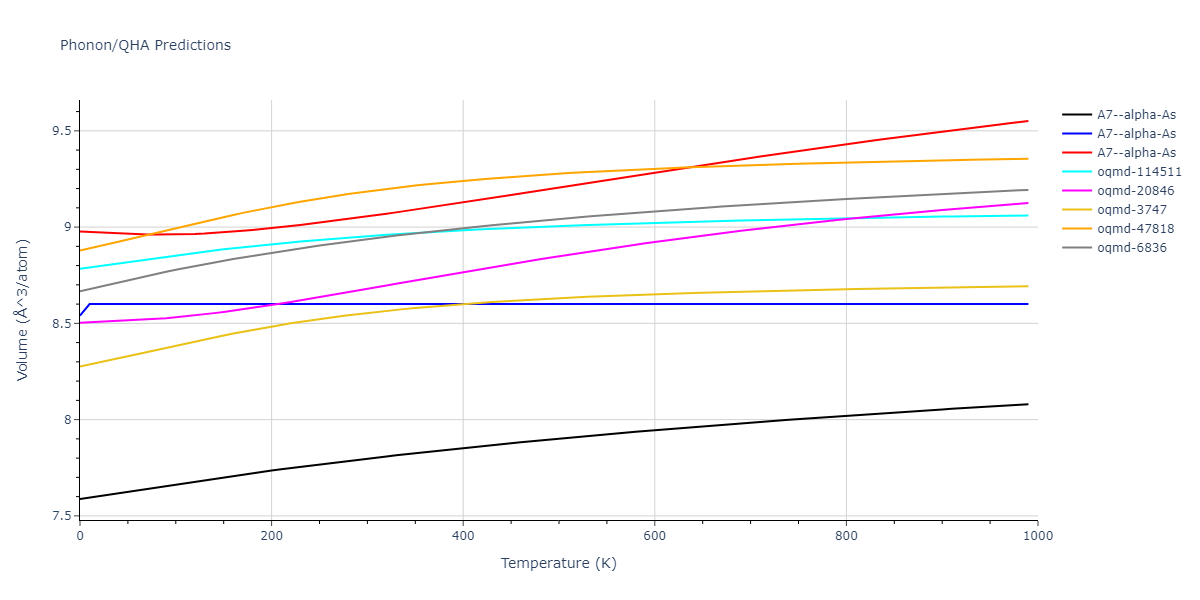
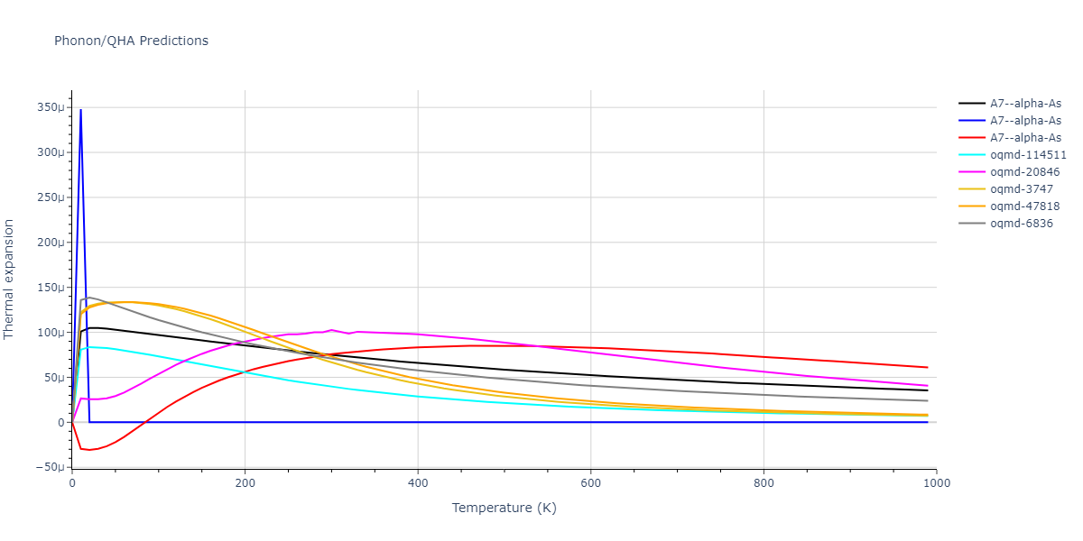
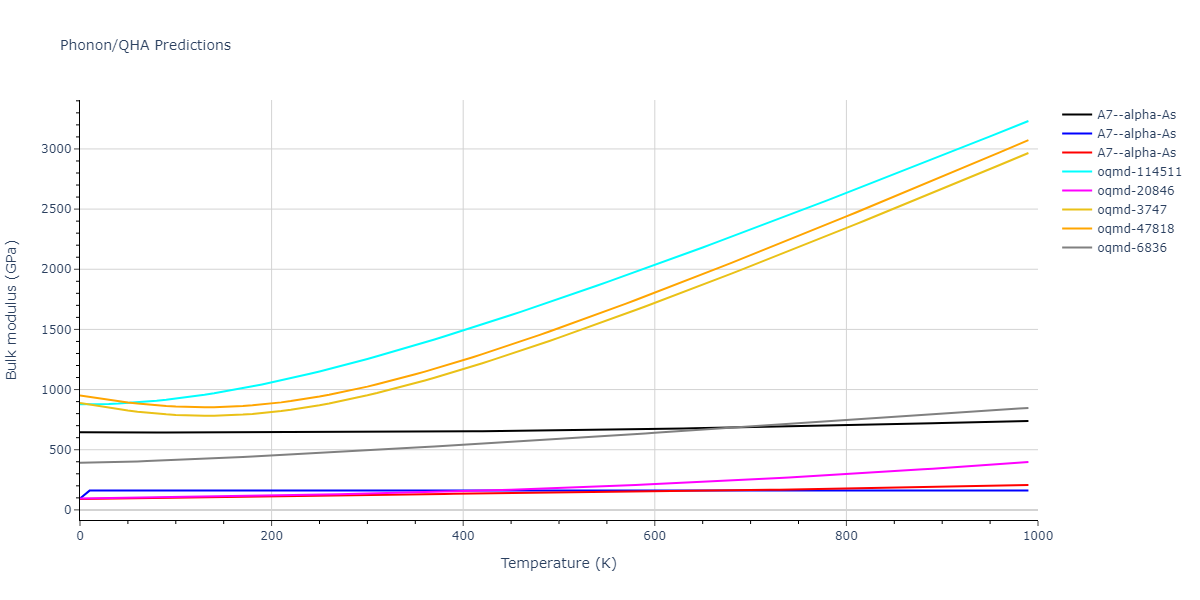
Free Surface Formation Energy Predictions
Static free surface formation energies are displayed for select crystals. The values displayed here are obtained by taking a perfect periodic bulk crystal, slicing along a crystallographic plane, and using force minimization to statically relax the surfaces. The free surface formation energy is computed by comparing the energy of the defect system to the bulk system and dividing by the total surface area created by the cut.
The calculation method used is available as the iprPy surface_energy_static calculation method.
Notes and Disclaimers:
- These values are meant to be guidelines for comparing potentials, not the absolute values for any potential's properties. Values listed here may change if the calculation methods are updated due to improvements/corrections. Variations in the values may occur for variations in calculation methods, simulation software and implementations of the interatomic potentials.
- The calculation only performs straight cuts along crystallographic planes and static relaxations. Lower energy configurations may exist that require atomic restructuring of the surfaces.
- Multiple values may be listed for a given plane followed by a number indicating different unique atomic planar cuts for the same theoretical plane.
- NIST disclaimer
Version Information:
- 2019-11-14. Calculations for the alternate #2 plane slices are now different from the #1 plane slices.
- 2019-08-07. Data added.
| Surface | γfs (mJ/m2) |
|---|---|
| (111) | 1363.48 |
| (332) | 1547.91 |
| (322) | 1571.83 |
| (100) | 1621.83 |
| (221) | 1633.75 |
| (211) | 1683.58 |
| (331) | 1708.07 |
| (311) | 1781.62 |
| (321) | 1805.89 |
| (110) | 1808.51 |
| (310) | 1882.39 |
| (320) | 1910.00 |
| (210) | 1941.16 |
| Surface | γfs (mJ/m2) |
|---|---|
| (211) 2 | 1298.83 |
| (210) | 1326.21 |
| (332) 2 | 1357.51 |
| (311) | 1375.51 |
| (321) 2 | 1388.99 |
| (100) | 1391.76 |
| (221) | 1400.80 |
| (321) 1 | 1402.61 |
| (111) | 1403.73 |
| (322) | 1424.74 |
| (331) | 1443.80 |
| (320) | 1451.84 |
| (310) | 1461.37 |
| (332) 1 | 1477.45 |
| (211) 1 | 1502.54 |
| (110) | 1561.20 |
| Surface | γfs (mJ/m2) |
|---|---|
| (110) | 1350.08 |
| (320) | 1516.00 |
| (321) | 1565.39 |
| (331) | 1587.27 |
| (210) | 1595.01 |
| (211) | 1630.70 |
| (100) | 1632.68 |
| (310) | 1663.18 |
| (221) | 1676.20 |
| (311) | 1720.85 |
| (322) | 1732.17 |
| (332) | 1745.15 |
| (111) | 1807.74 |
| Surface | γfs (mJ/m2) |
|---|---|
| (111) | -13772.51 |
| (201) | -13135.51 |
| (100) | 1041.64 |
| (101) 1 | 1324.70 |
| (211) 1 | 1345.60 |
| (112) | 1368.10 |
| (211) 2 | 1526.34 |
| (001) | 1556.23 |
| (110) | 1646.00 |
| (101) 2 | 2238.58 |
Stacking Fault Energy Predictions
Stacking fault energy plots and maps are displayed for select crystals. The values are computed by
- Starting with a bulk crystal system
- Creating a free surface along one of the system's periodic boundaries and using force minimization to relax it
- The system is sliced in half along a crystallographic plane parallel to the free surface. One half of the system is shifted relative to the other
- The atoms in the shifted system are allowed to relax only in the direction normal to the shifting plane
- The stacking fault energy for a given shift is computed by comparing the energy of the system before and after applying the shift, and dividing by the area of the fault plane
The calculation method used is available as the iprPy stacking_fault_map_2D calculation method.
Notes and Disclaimers:
- These values are meant to be guidelines for comparing potentials, not the absolute values for any potential's properties. Values listed here may change if the calculation methods are updated due to improvements/corrections. Variations in the values may occur for variations in calculation methods, simulation software and implementations of the interatomic potentials.
- Values between the measured points are interpolated and therefore may not perfectly capture minima and maxima.
- Multiple values may be listed for a given plane followed by a number indicating different unique atomic planar cuts for the same theoretical plane.
- NIST disclaimer
Version Information:
- 2022-06-28. Table added for intrinsic and unstable energies, and ideal shear stresses. Plots (and table) now ordered by the associated planes.
- 2019-11-14. Calculations for the alternate #2 plane slices are now different from the #1 plane slices. The 1D plotting vectors have been changed to avoid duplicates. Minor improvements to how the 2D plots are displayed.
- 2019-08-07. Plots added.
Stacking fault energies in mJ/m2 and ideal shears in GPa
| E_usf a/2 [0 -1 1] | 1564.43 |
| τ_ideal a/2 [0 -1 1] | 38.15 |
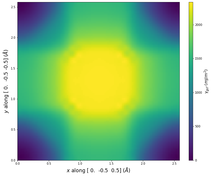
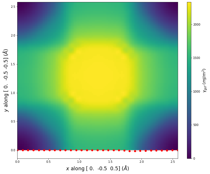
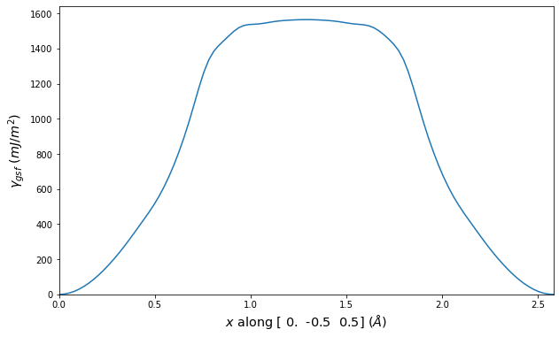
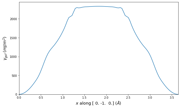
Stacking fault energies in mJ/m2 and ideal shears in GPa
| E_isf | -18.59 |
| E_usf a/2 [0 -1 1] | 270.52 |
| τ_ideal a/2 [0 -1 1] | 7.48 |
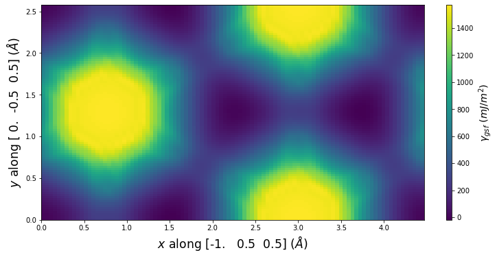
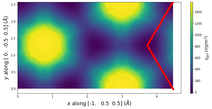
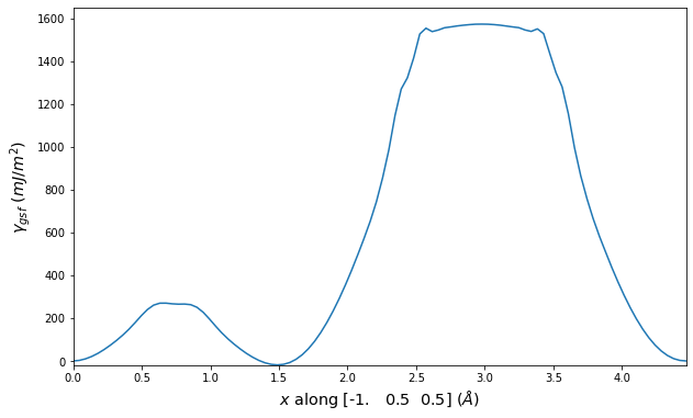
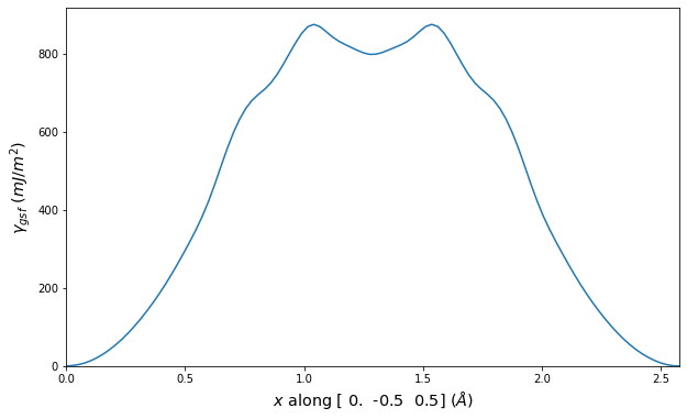
Stacking fault energies in mJ/m2 and ideal shears in GPa
| E_usf a/2 [-1 1 -1] | 901.22 |
| τ_ideal a/2 [-1 1 -1] | 14.30 |
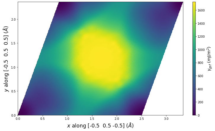

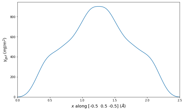

Stacking fault energies in mJ/m2 and ideal shears in GPa
| E_usf a/2 [-1 -1 1] | 1054.97 |
| τ_ideal a/2 [-1 -1 1] | 15.86 |
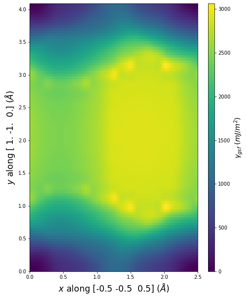


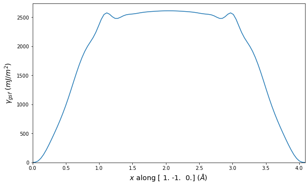
Stacking fault energies in mJ/m2 and ideal shears in GPa
| E_usf a/2 [-1 -1 1] | 1042.26 |
| τ_ideal a/2 [-1 -1 1] | 15.32 |

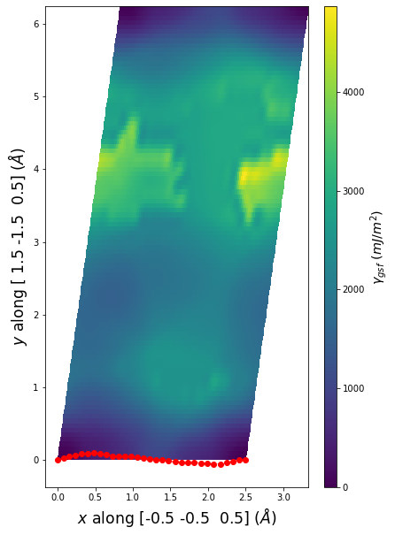
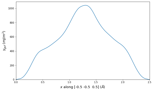
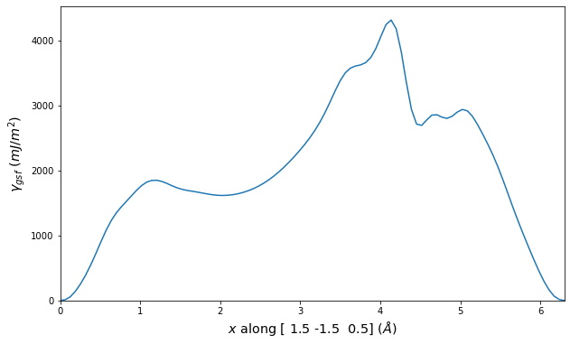
Point Defect Formation Energy Predictions
Static point defect formation energies, Ef, and elastic dipole tensors, pij, are displayed for select crystals. Relaxed defect configurations are obtained by taking a 12x12x12 supercell of a perfect periodic bulk crystal, inserting the point defect, and using force minimization to statically relax the atomic positions while keeping the system dimensions constant. Ef is computed by comparing the energy of the defect system to the same number of atoms in a perfect bulk crystal. pij is estimated as the difference in the system's global pressure with and without the defect multiplied by the system's volume.
Simple structural comparisons of the unrelaxed and relaxed defect configurations are used to help determine if the defect structure has relaxed to a different configuration. Relaxed structures that are identified as no longer consistent with the ideal defect definition are excluded from the table below. The only exception to this is if the lowest energy interstitial configuration does not coincide with a known ideal defect, its energies and pressure tensor are included under the listing "relaxed interstitial". The full list of calculation results including the transformed structures and the structural comparison values is included in the csv file available from the "Download raw data" link.
The calculation method used is available as the iprPy point_defect_static calculation method.
Notes and Disclaimers:
- These values are meant to be guidelines for comparing potentials, not the absolute values for any potential's properties. Values listed here may change if the calculation methods are updated due to improvements/corrections. Variations in the values may occur for changes in calculation methods, simulation software and implementations of the interatomic potentials.
- The computed formation energy and elastic dipole tensor values are sensitive to the size of the system used. The 12x12x12 supercell size was selected as it should provide a decent approximation of the true bulk values.
- The tests for identifying configuration relaxations are not guaranteed to be comprehensive or suitable for all point defect types. The table only shows the point defects that are consistent with the ideal configurations for that defect type, and the lowest energy interstitial.
- The "relaxed interstitial" label indicates that the structure is not consistent with any of the known ideal interstitial configurations. No information is provided as to what that relaxed strucutre is, whether it is an unknown structure, a "near"-ideal defect, or a collapse to amorphous.
- NIST disclaimer
| Point Defect | Ef (eV) | p11 (eV) | p22 (eV) | p33 (eV) | p12 (eV) | p13 (eV) | p23 (eV) |
|---|---|---|---|---|---|---|---|
| vacancy | 1.919 | -2.935 | -2.935 | -2.935 | 0.000 | -0.000 | -0.000 |
| 1nn divacancy | 3.533 | -5.657 | -5.509 | -5.509 | -0.000 | -0.000 | -0.084 |
| 100 dumbbell | 3.567 | 19.646 | 19.646 | 21.691 | 0.000 | 0.000 | 0.000 |
| 2nn divacancy | 3.865 | -5.931 | -5.931 | -5.916 | 0.000 | -0.000 | -0.000 |
| tetrahedral interstitial | 4.042 | 20.745 | 20.745 | 20.745 | 0.000 | 0.000 | -0.000 |
| octahedral interstitial | 4.624 | 19.622 | 19.622 | 19.622 | 0.000 | -0.000 | -0.000 |
| Point Defect | Ef (eV) | p11 (eV) | p22 (eV) | p33 (eV) | p12 (eV) | p13 (eV) | p23 (eV) |
|---|---|---|---|---|---|---|---|
| vacancy | 1.565 | -4.524 | -4.524 | -4.524 | -0.000 | -0.000 | 0.000 |
| 2nn divacancy | 2.937 | -9.555 | -9.555 | -10.743 | -0.000 | 0.000 | -0.000 |
| 1nn divacancy | 2.995 | -7.437 | -7.437 | -7.437 | 0.637 | 0.637 | 0.637 |
| 110 dumbbell | 4.525 | 17.991 | 14.283 | 14.283 | -0.000 | 0.000 | 6.029 |
| 111 dumbbell | 4.783 | 18.489 | 18.489 | 18.489 | 9.247 | 9.247 | 9.247 |
| tetrahedral interstitial | 5.252 | 19.353 | 10.615 | 19.353 | 0.000 | -0.000 | -0.000 |
| 100 dumbbell | 5.785 | 17.352 | 17.352 | 24.906 | 0.000 | -0.000 | 0.000 |
Dislocation Monopole Structures
Plots of the atomic structure of dislocation cores are shown here. The dislocations were constructed using dislocation monopole configurations in which a straight dislocation is created in the center of the system using anisotropic elasticity and the elastic constants computed above. A cylindrical region centered around the dislocation is allowed to relax while the remaining atoms are held fixed. The relaxation consists of 1 million NVT steps at 10 K followed by an energy/force minimization. The final plots show the atomic configuration near the center of the monopole system, and display differential displacement arrows and Nye tensor color maps that are both taken with respect to the Burgers vector direction.
These plots show a wide range of final structures, some corresponding to expected dislocation structures and others not. While the characterizations are dislocation-type dependent, some general classification guidelines are listed here.
- Planar dislocations exist on a single slip plane, which results in a grouping of large differential displacement arrows between two atomic rows. All edge dislocations and some screw dislocations may be planar dislocations.
- Non-planar dislocations are screw dislocations that are positioned at the intersection of more than one slip plane. This results in the differential displacement arrows circling the position of the dislocation core. These core structures often have rotational symmetry due to the intersecting planes.
- The plotted atomic positions are also useful for characterizing the final configuration. For screw dislocations, the atomic projections should match projections in the bulk crystal if the crystal has not transformed. For edge dislocations, the projections should be the bulk projections with the extra half-plane of atoms directly above the dislocation core.
- Images in which the atomic positions look correct but no large differential displacement arrows are observed are likely the result of the dislocation gliding out of view during relaxation.
- Phase transformations are identified by large differential displacement arrows spread out in both plot directions, often across the whole image. Additionally, the atomic position projections will likely not correspond to what is expected.
- Twins typically appear as a long line of large differential displacement arrows along a single plane. Note that twins can nucleate phase transformations so the distinction between the two is not always clear.
The calculation method used is available as the iprPy dislocation_monopole calculation method.
Links are provided above the images allowing for users to download the final defect configuration and a corresponding defect-free configuration if they wish to further analyze the structures or use them for subsequent simulations.
Notes and Disclaimers:
- While the general dislocation monopole method is universal to all dislocations, these calculations rely on dislocation-type specific atomic configuration sizes and differential displacement/Nye tensor settings. For the system size, the specific super cell multipliers vary based on the crystal and crystal vector orientations, but the sizes are always selected to minimize the length along the dislocation line and attempt to make the two other box dimensions similar. For the structure analysis tools, both are sensitive to the cutoff distance used to identify neighbors, and both have some method-specific parameters. Where known, the settings used here correspond to the most common ones used in literature.
- For bcc dislocations, the differential displacement vectors shown here are "wrapped" in that if their magnitudes exceed b/2 then a value of b is added/subtracted to wrap the vector back around. This convention reveals the dislocation's structure and location without showing the slip history.
- NIST disclaimer
Version Information:
- 2025-08-07. Plots first added.
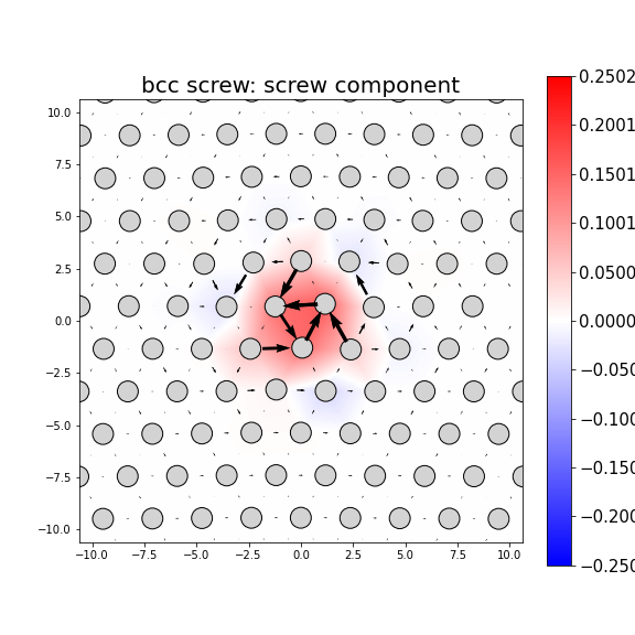
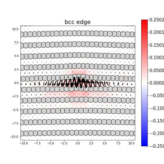
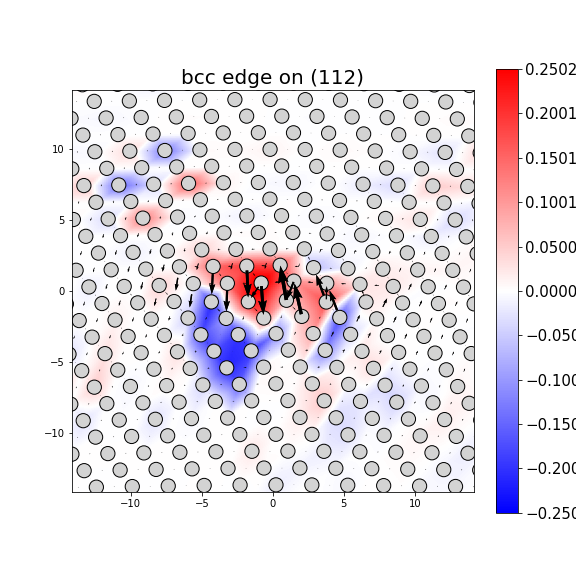
MD Solid Property Predictions
Plots of lattice and elastic constants are shown as a function of temperature. The 0K points were taken from the Crystal Structure Predictions and the Elastic Constants Predictions sections above for the unique crystal structures relaxed with the "dynamic" method. Starting from the 0 K relaxed crystal unit cells, supercell systems are created by replicating all three dimensions by the same multiplier to achieve at least 4000 atoms. The systems are then relaxed at 50 K and zero pressure using 1 million NPT steps. Lattice constants are estimated by averaging the measured box dimensions. Temperatures are iteratively increased by 50 K, with each subsequent relaxation calculation starting from the final atomic configuration at the previous temperature and relaxing for another 1 million steps.
The elastic constants are calculated using the deformation–fluctuation hybrid method. Starting from the final atomic configurations of the dynamic relaxations, the system is allowed to evolve at constant volume with a Langevin thermostat. The Born matrix is computed during this run by evaluating how the atomic forces would vary due to applied linear strain fields. The elastic constants can then be estimated using the averaged Born matrix values and the averaged stresses on the system.
The calculation methods used are available as the iprPy relax_dynamic and elastic_constants_dynamic calculation methods.
Clicking on the image of a plot will open an interactive version of it in a new tab. The underlying data for the plots can be downloaded by clicking on the links above each plot.
Notes and Disclaimers:
- The maximum temperature shown for a crystal either corresponds to the maximum value that has been computed so far, or the maximum value that the structure is believed to have remained untransformed. The unstable/transformation temperature identification is mostly automated and can miss transitions not associated with large discontinuities in property values with changing temperature.
- For succinctness, the elastic constants displayed here are averaged according to the 0 K structure's crystal symmetry family. If the structures deviate from the expected symmetry at higher temperatures, the values may not be valid. Raw results are available for verification if requested.
- NIST disclaimer
Version Information:
- 2025-08-07. Plots added.
Click on plot to load interactive version
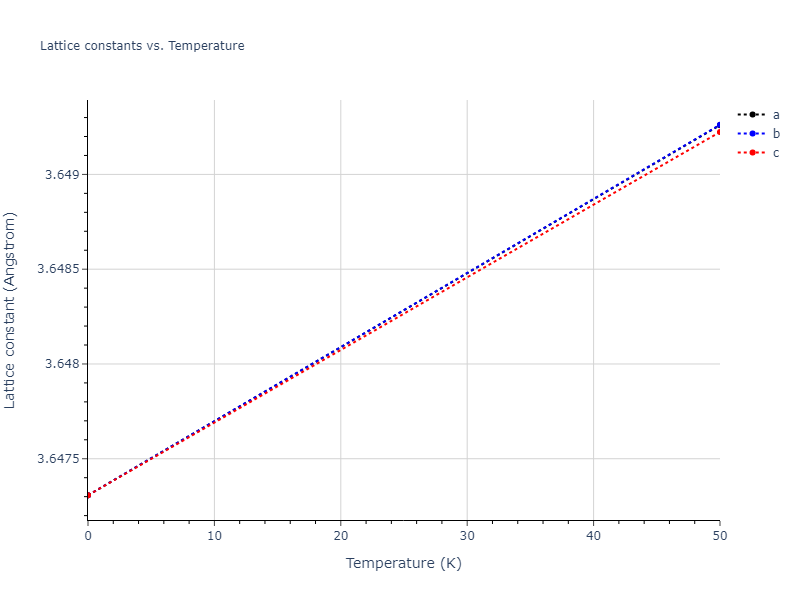
Click on plot to load interactive version
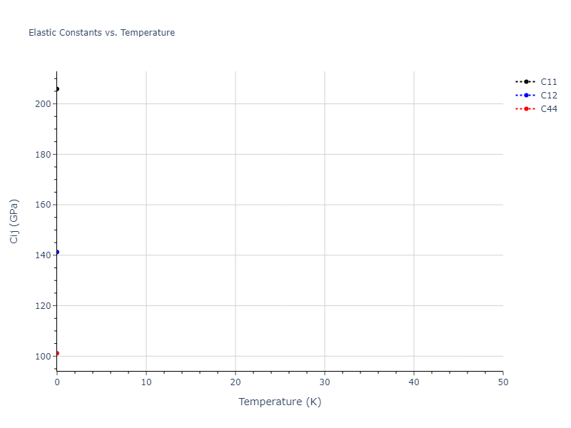
Click on plot to load interactive version
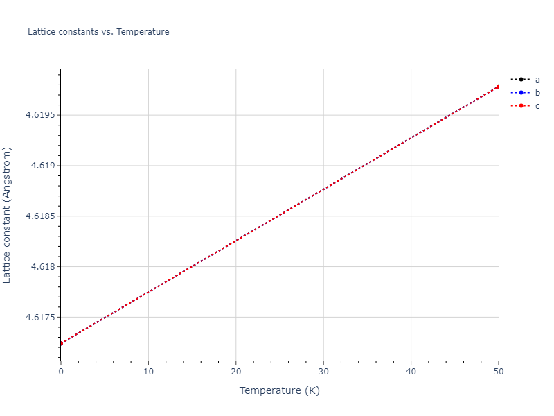
Click on plot to load interactive version

Click on plot to load interactive version

Click on plot to load interactive version
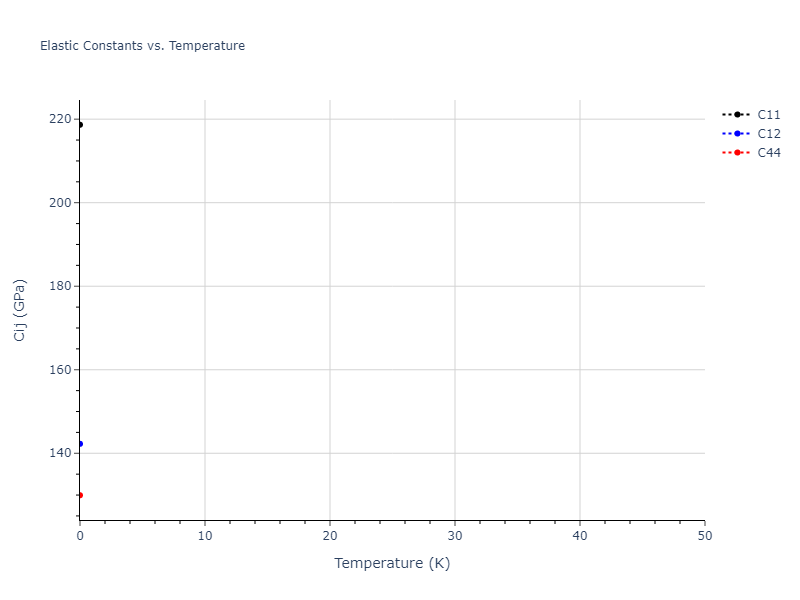
Click on plot to load interactive version

Click on plot to load interactive version
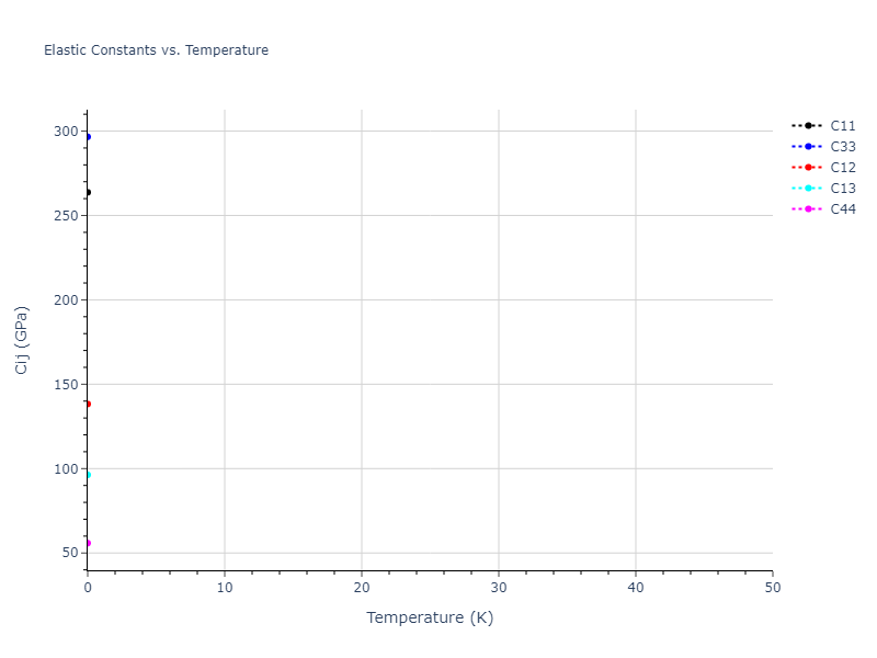
Click on plot to load interactive version

Click on plot to load interactive version

Click on plot to load interactive version
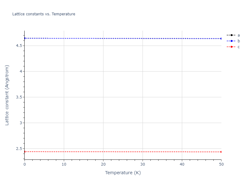
Click on plot to load interactive version

Click on plot to load interactive version
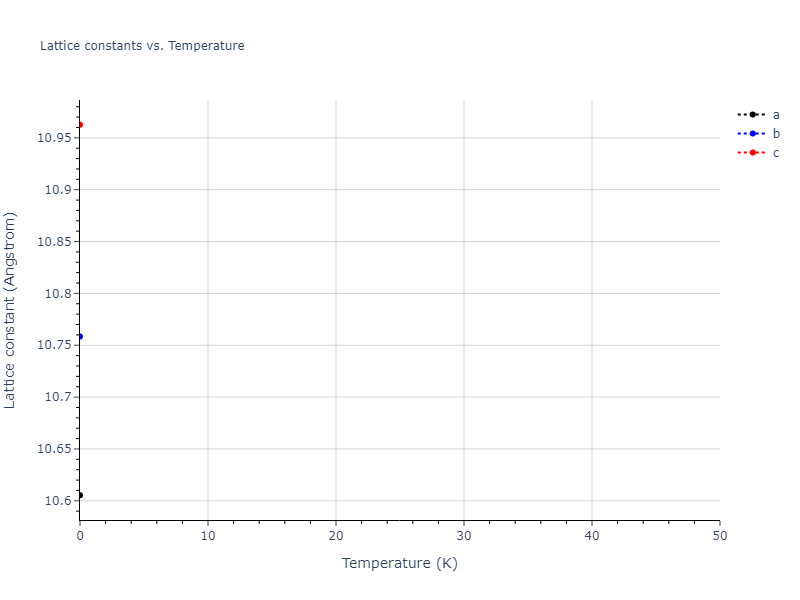
Click on plot to load interactive version
Click on plot to load interactive version
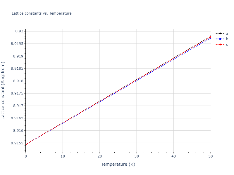
Click on plot to load interactive version

Click on plot to load interactive version
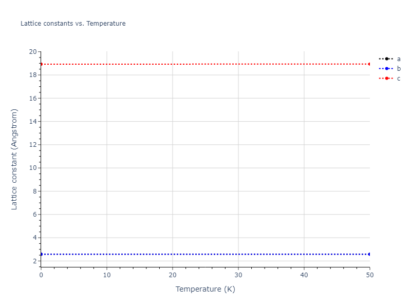
Click on plot to load interactive version

Click on plot to load interactive version
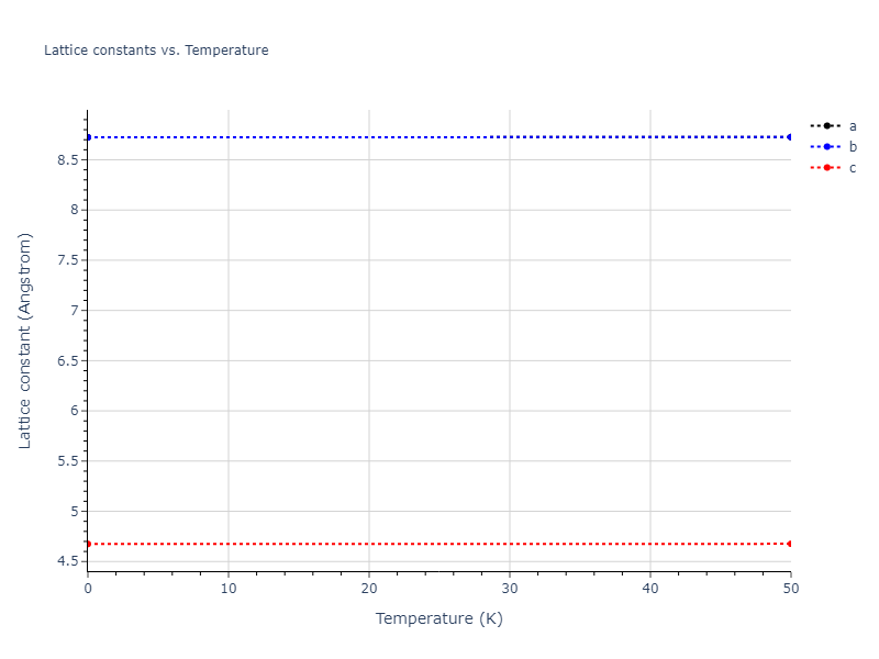
Click on plot to load interactive version
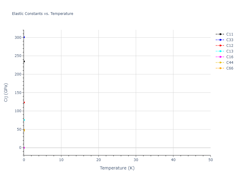
Click on plot to load interactive version

Click on plot to load interactive version

Click on plot to load interactive version

Click on plot to load interactive version

Click on plot to load interactive version
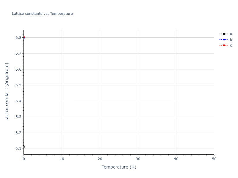
Click on plot to load interactive version

Click on plot to load interactive version

Click on plot to load interactive version
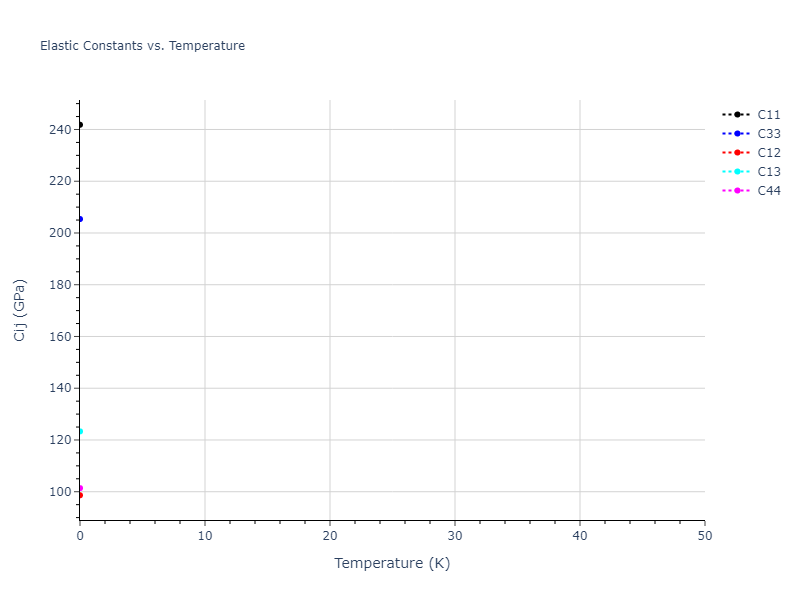
Click on plot to load interactive version

Click on plot to load interactive version

Click on plot to load interactive version

Click on plot to load interactive version

Click on plot to load interactive version

Click on plot to load interactive version

Click on plot to load interactive version

Click on plot to load interactive version

Click on plot to load interactive version

Click on plot to load interactive version

Click on plot to load interactive version

Click on plot to load interactive version

Click on plot to load interactive version
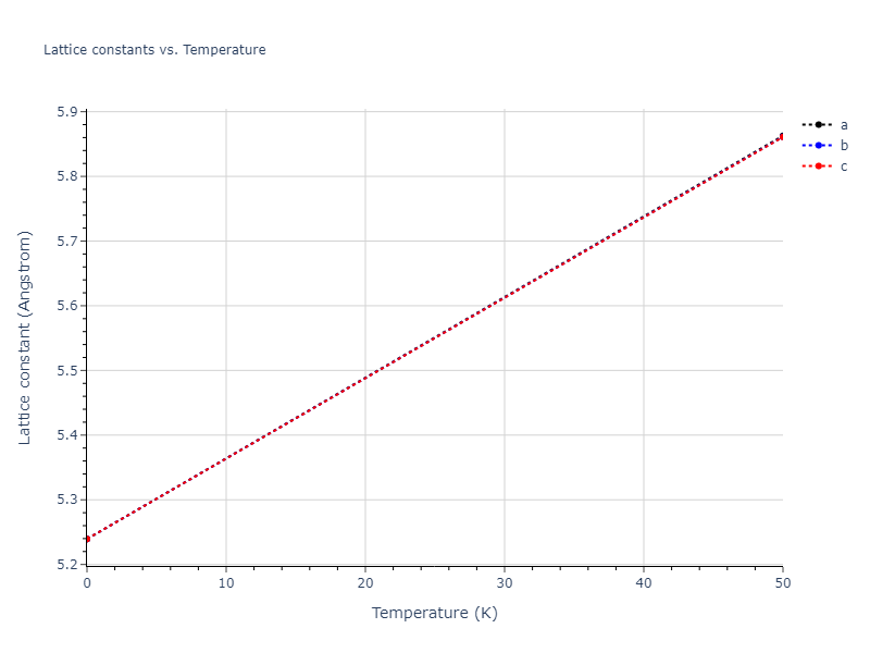
Click on plot to load interactive version

Click on plot to load interactive version

Click on plot to load interactive version

Click on plot to load interactive version

Click on plot to load interactive version
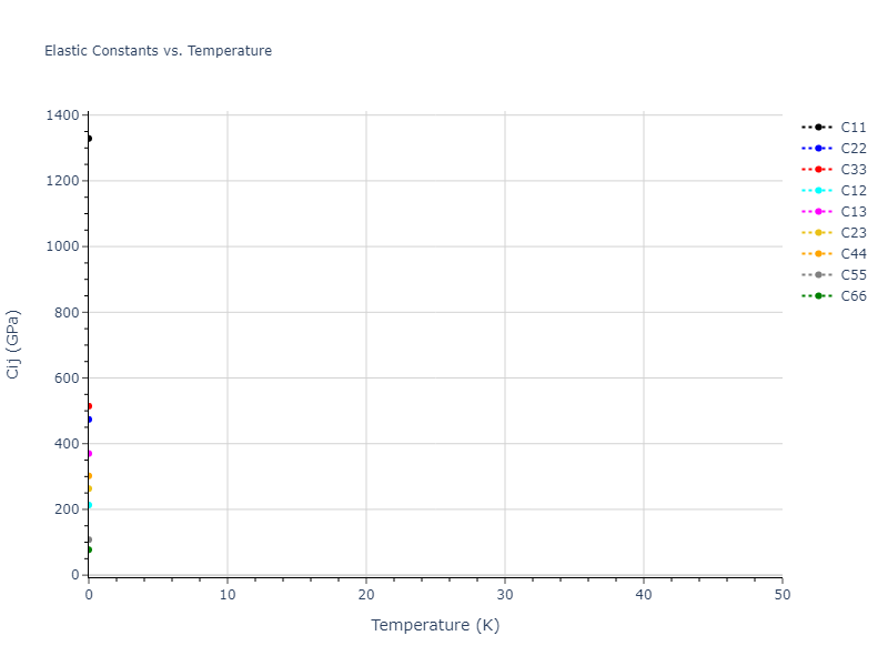
Click on plot to load interactive version

Click on plot to load interactive version

Click on plot to load interactive version

Click on plot to load interactive version

Click on plot to load interactive version

Click on plot to load interactive version

Click on plot to load interactive version

Click on plot to load interactive version

Click on plot to load interactive version

Click on plot to load interactive version

Click on plot to load interactive version
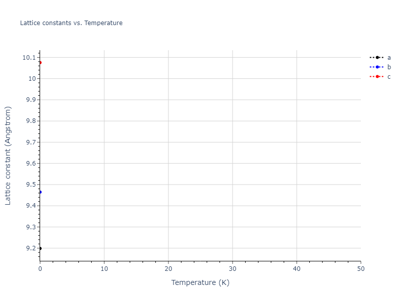
Click on plot to load interactive version

Click on plot to load interactive version

Click on plot to load interactive version

Click on plot to load interactive version

Click on plot to load interactive version
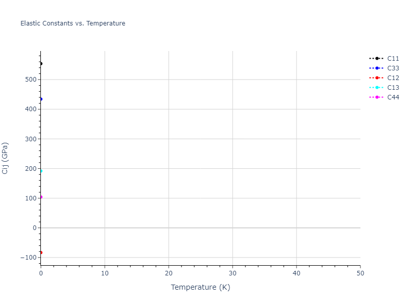
Click on plot to load interactive version
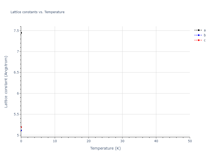
Click on plot to load interactive version
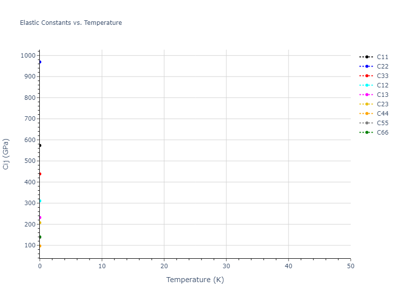
Click on plot to load interactive version

Click on plot to load interactive version

Click on plot to load interactive version

Click on plot to load interactive version

Click on plot to load interactive version

Click on plot to load interactive version
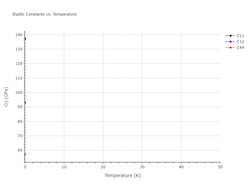
Click on plot to load interactive version

Click on plot to load interactive version

Click on plot to load interactive version

Click on plot to load interactive version
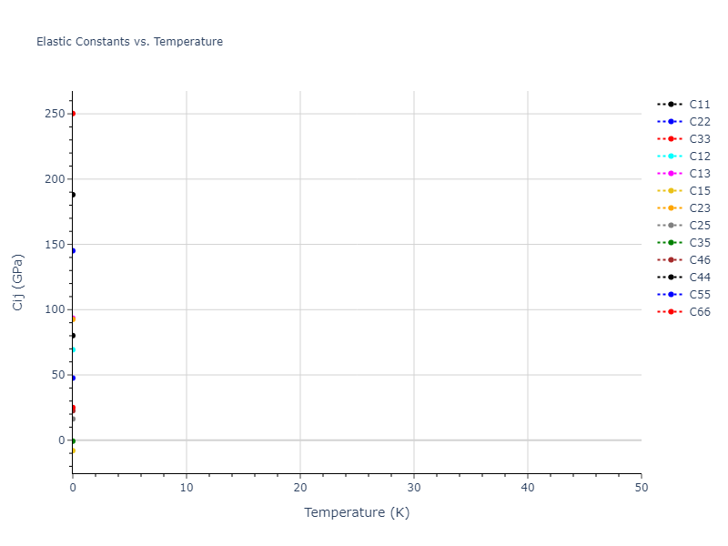
Click on plot to load interactive version
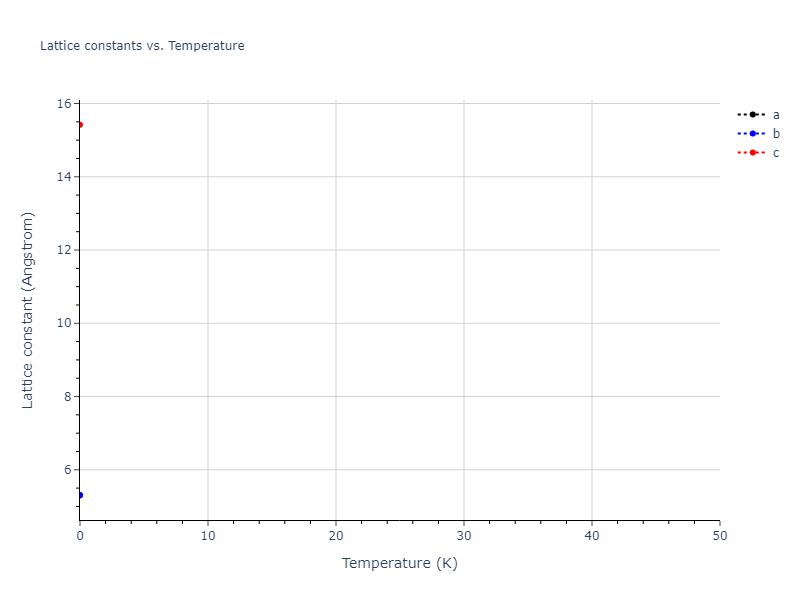
Click on plot to load interactive version
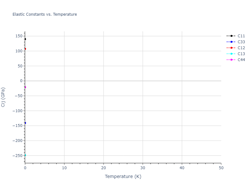
Click on plot to load interactive version

Click on plot to load interactive version
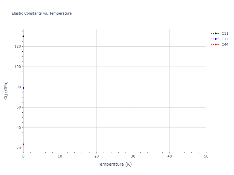
Click on plot to load interactive version

Click on plot to load interactive version

Click on plot to load interactive version
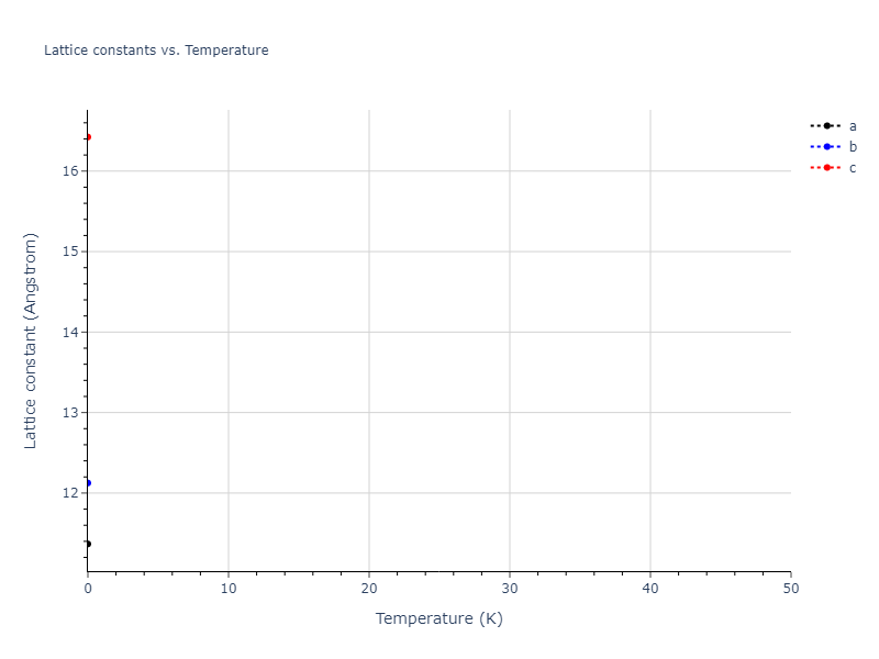
Click on plot to load interactive version

Click on plot to load interactive version
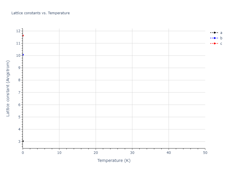
Click on plot to load interactive version
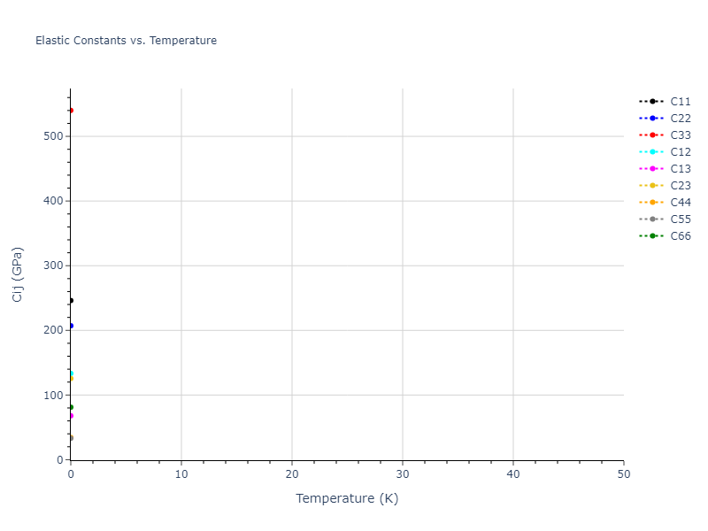
Click on plot to load interactive version

Click on plot to load interactive version

Click on plot to load interactive version
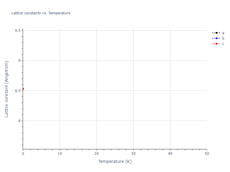
Click on plot to load interactive version
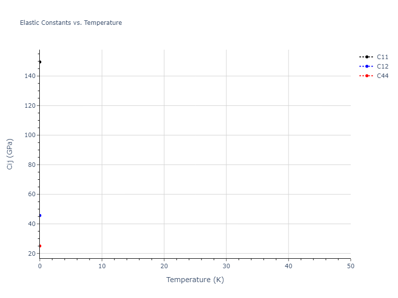
Click on plot to load interactive version
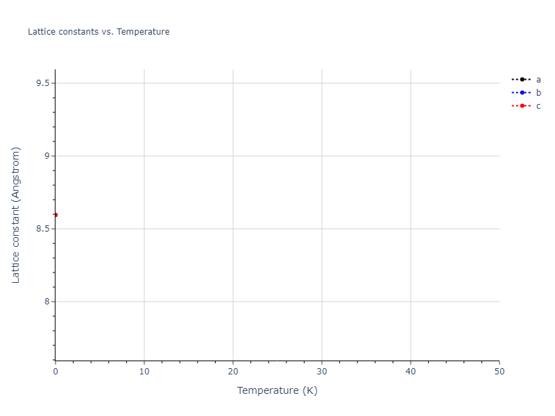
Click on plot to load interactive version

Click on plot to load interactive version

Click on plot to load interactive version

Click on plot to load interactive version
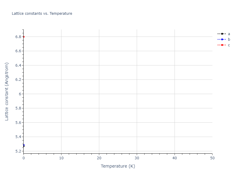
Click on plot to load interactive version

Click on plot to load interactive version

Click on plot to load interactive version

Click on plot to load interactive version
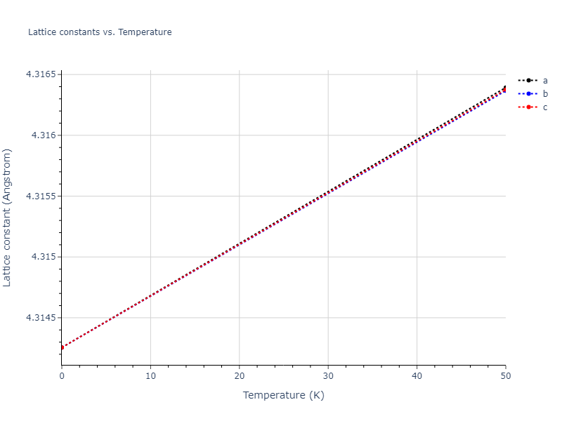
Click on plot to load interactive version
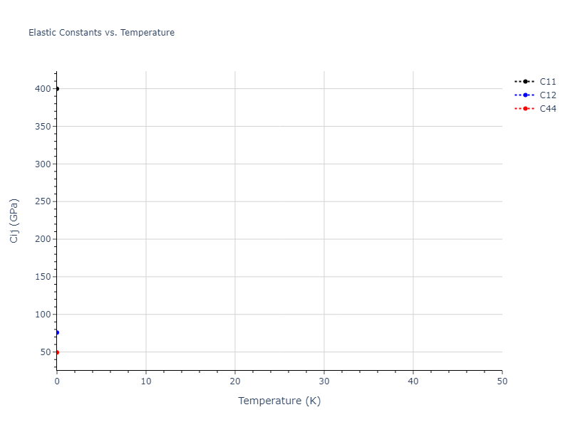
Click on plot to load interactive version
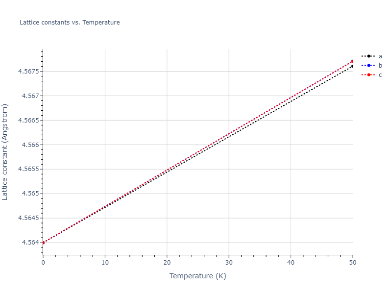
Click on plot to load interactive version
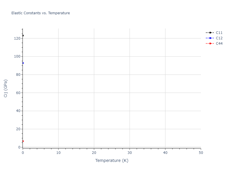
Click on plot to load interactive version

Click on plot to load interactive version

Click on plot to load interactive version

Click on plot to load interactive version

Click on plot to load interactive version

Click on plot to load interactive version
Click on plot to load interactive version
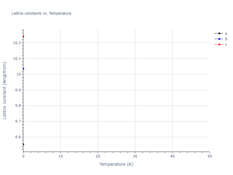
Click on plot to load interactive version

Click on plot to load interactive version

Click on plot to load interactive version

Click on plot to load interactive version
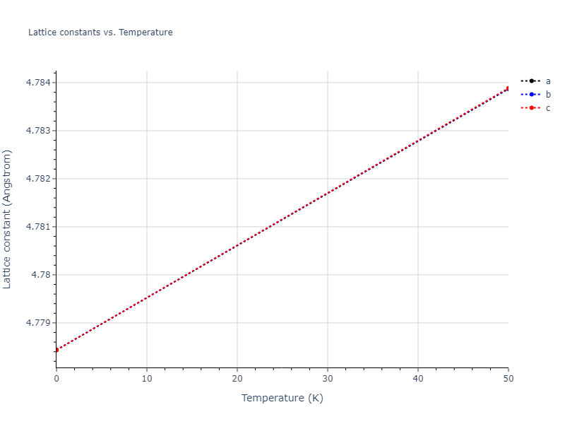
Click on plot to load interactive version
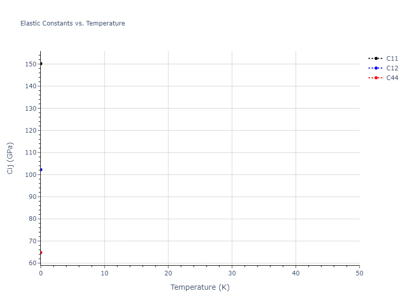
Click on plot to load interactive version
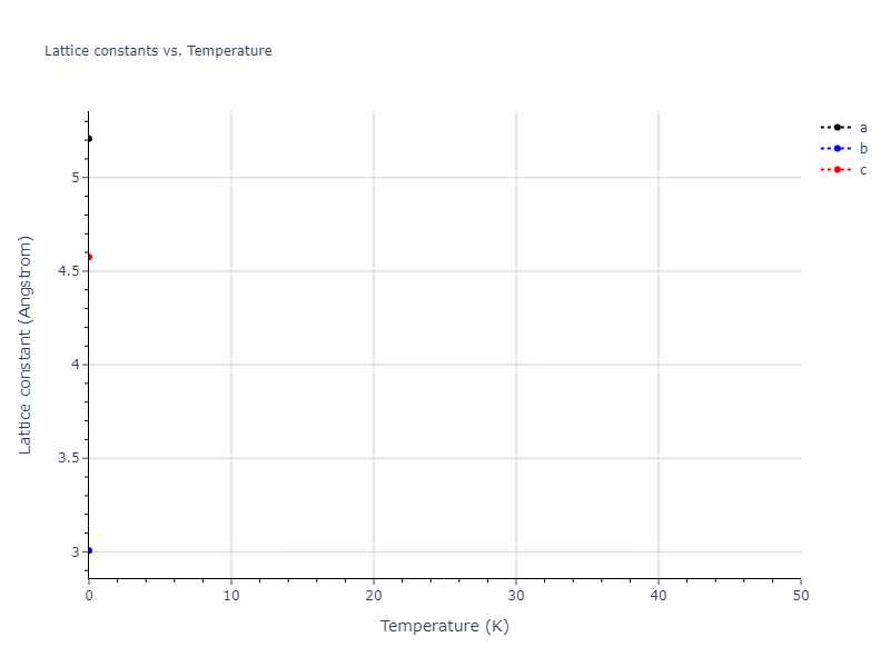
Click on plot to load interactive version

Click on plot to load interactive version

Click on plot to load interactive version
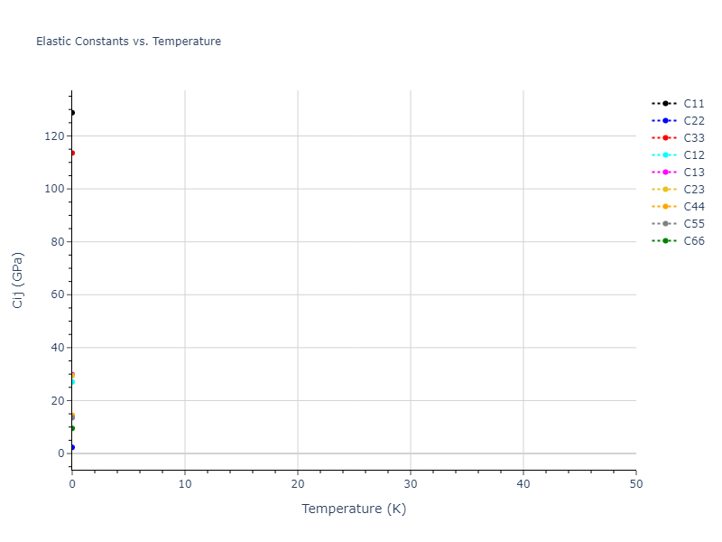
Click on plot to load interactive version

Click on plot to load interactive version

Click on plot to load interactive version
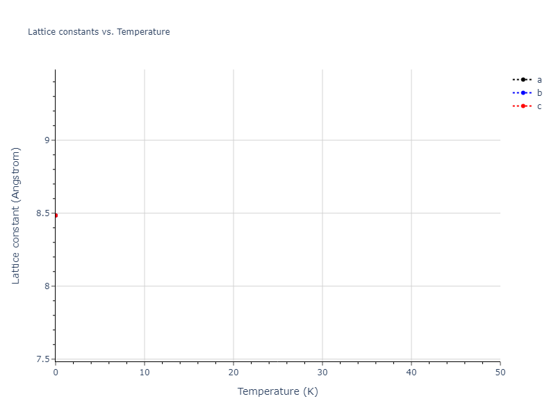
Click on plot to load interactive version

Click on plot to load interactive version

Click on plot to load interactive version

Click on plot to load interactive version

Click on plot to load interactive version
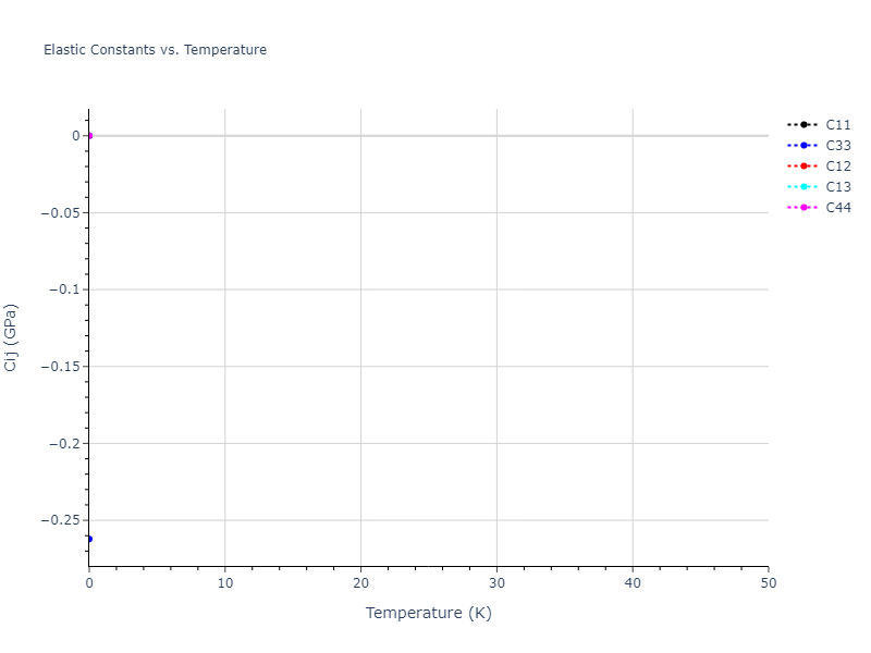
Click on plot to load interactive version

Click on plot to load interactive version
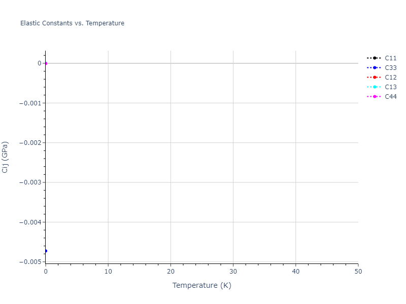
Click on plot to load interactive version

Click on plot to load interactive version

Click on plot to load interactive version

Click on plot to load interactive version

Click on plot to load interactive version

Click on plot to load interactive version

Click on plot to load interactive version
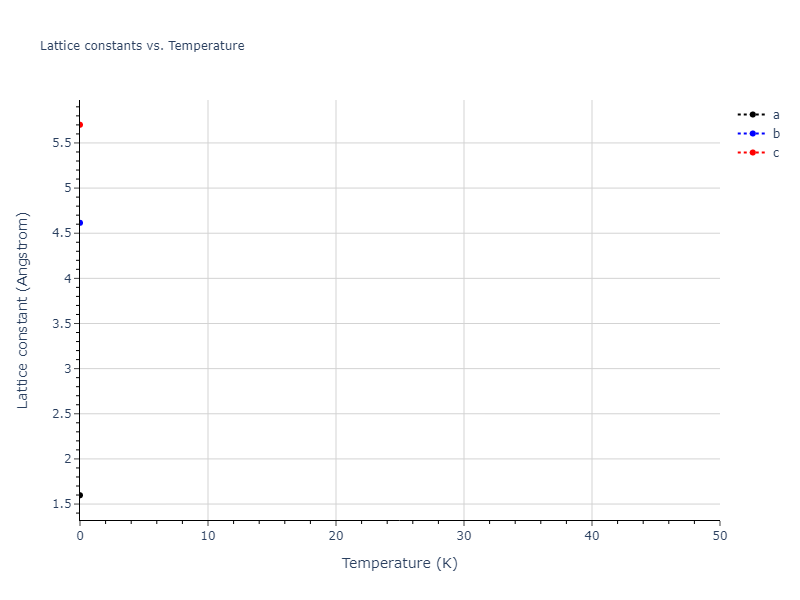
Click on plot to load interactive version
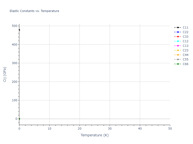
Click on plot to load interactive version

Click on plot to load interactive version
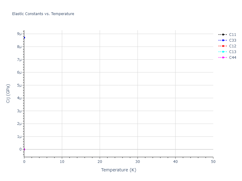
Click on plot to load interactive version

Click on plot to load interactive version

Click on plot to load interactive version
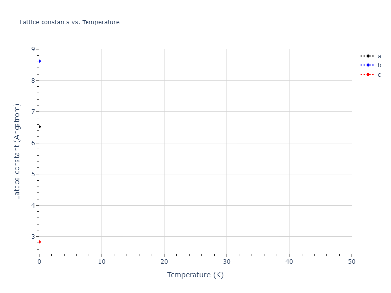
Click on plot to load interactive version

Click on plot to load interactive version
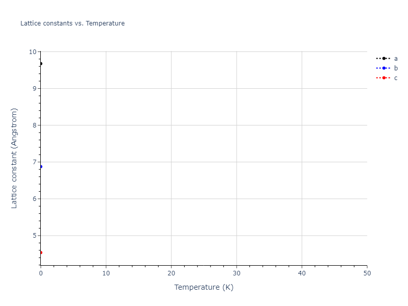
Click on plot to load interactive version

Click on plot to load interactive version
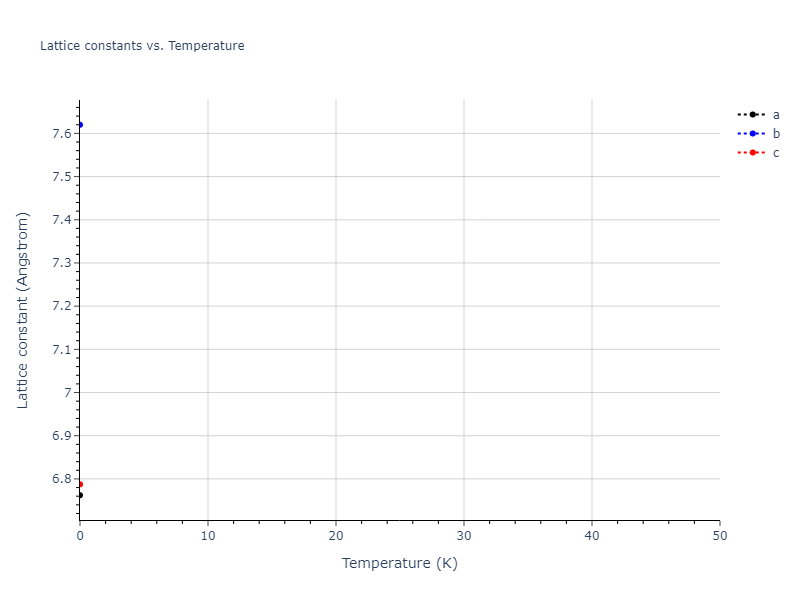
Click on plot to load interactive version
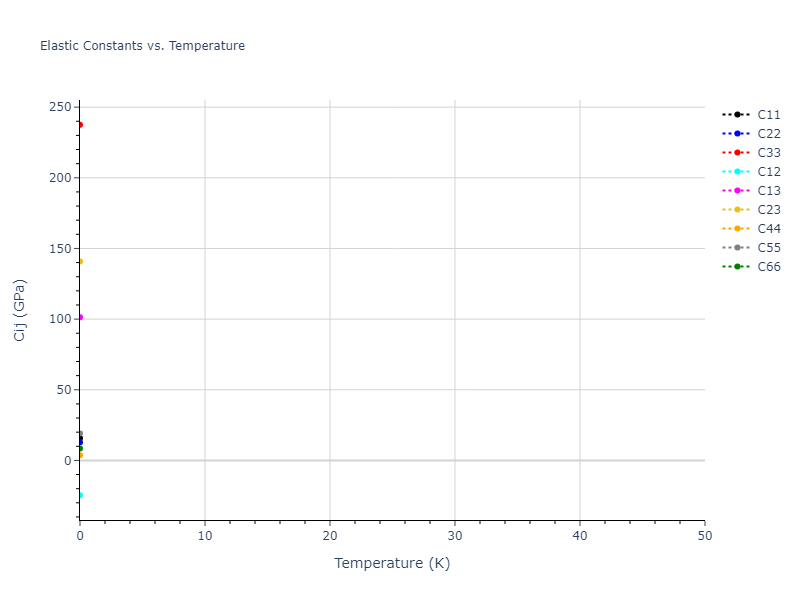
Click on plot to load interactive version

Click on plot to load interactive version
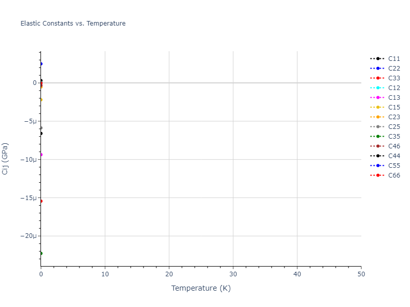
Click on plot to load interactive version

Click on plot to load interactive version
Click on plot to load interactive version
Click on plot to load interactive version

Click on plot to load interactive version

Click on plot to load interactive version
Click on plot to load interactive version
Click on plot to load interactive version
Click on plot to load interactive version
Click on plot to load interactive version
Click on plot to load interactive version
Click on plot to load interactive version
Click on plot to load interactive version
Click on plot to load interactive version

MD Liquid Property Predictions
Plots of radial distribution functions at different temperatures and the temperature-dependent diffusion and viscosity are shown here for elemental liquids. Melt phases are constructed by starting with a 10x10x10 fcc super cell and relaxing with 50,000 NPT steps at zero pressure and a high melting temperature (3000 K for most potentials and elements). Following the melt, liquid structures are relaxed by running NPT for 10,000 steps over which the temperature is dropped by 50 K, then 50,000 NPT at the target temperature to estimate the equilibrium volume, followed by 20,000 NVT steps at the averaged equilibrium volume and target temperature. Structures from the NVT run are sampled to compute the radial distribution function of the liquid at the corresponding temperature.
The final relaxed configurations at each temperature explored are used as the initial configurations for the diffusion and viscosity calculations. For diffusion, the system is integrated for 100 runs of 2,000 NVT steps during which both the mean squared displacement (MSD) and the velocity auto correlation function (VACF) are computed. From these simulations, three estimates of diffusion are computed: one from the MSD of the full 200,000 step run, one in which the MSD is reset for each short run and then averaged, and one from the VACF computed for each short run and averaged. For viscosity, the Green-Kubo method is used which is evaluated during a 1 million step NVT run.
The calculation methods used are available as the iprPy relax_liquid_redo, diffusion_liquid, and viscosity_green_kubo calculation methods.
Clicking on the image of a plot will open an interactive version of it in a new tab. The underlying data for the plots can be downloaded by clicking on the links above each plot.
Notes and Disclaimers:
- The current liquid relaxation has some known issues, and therefore may be recalculated with an improved method later. Most notably, the unconstrained NPT relaxation may lead to one of the periodic dimensions becoming quite small which can negatively affect the simulations and property calculations. Additionally, the relaxations likely need to be longer to reduce the error associated with the measured volume and energy values.
- Values are only displayed down to the last temperature currently calculated, or the last temperature at which the system is believed to remain liquid until the end of all simulations. The transformation temperature is estimated by looking at discontinuities in the measured property values and may incorrectly predict a phase to still be liquid if the discontinuities are small.
- The three diffusion estimates provide a range of prediction values. For MSD, the longer the run the more likely it is that a small number of atoms will diffuse much farther than the rest, which skews the squared displacement higher.
- NIST disclaimer
Version Information:
- 2025-08-07. Plots added. Data should be thought of as preliminary as results may be recalculated later.
Click on plot to load interactive version
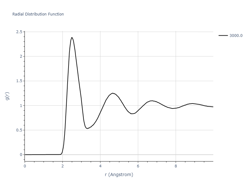
Click on plot to load interactive version
Click on plot to load interactive version
MD Thermodynamic Predictions
Plots of internal energy, Gibbs free energy, entropy, heat capacity and volume are shown here as a function of temperature for various crystal structures and liquid phases. The included crystal structures correspond to those in the Solid Structures vs. Temperature section, and the liquid phases to those in the Liquid Properties section. Internal energy and volume are taken from the associated structure relaxations mentioned in those previous sections. Constant pressure heat capacity is estimated using 3-point numerical derivatives of enthalpy versus temperature. Note that since all simulations done here are at 0 pressure, internal energy and enthalpy are equivalent.
The Gibbs energies of the phases are estimated using thermodynamic integration between the interatomic potential in question and a simpler model with known Gibbs free energy values. For solids, the reference model is an Einstein solid, while for liquids it is the Uhlenbeck-Ford potential. Besides a short run at the start of the solid calculations to estimate Einstein model spring constants, the two calculations proceed similarly. Starting with the final relaxation configurations, the systems are stabilized for 25,000 steps. Then, over the next 50,000 steps the potential is swapped out for the reference potential. The system is then stabilized for another 25,000 steps with the reference model before a reverse swap of 50,000 steps is performed. The simulation ends with one final 25,000 step stabilization period. From the simulation, the irreversible work of transformation is estimated and used to compute the absolute Gibbs free energy of the target phase and potential relative to the reference potential. Entropy is estimated as the difference in enthalpy and Gibbs free energy and divided by temperature.
The calculation methods used are available as the iprPy relax_dynamic, relax_liquid_redo, free_energy, and free_energy_liquid calculation methods.
Clicking on the image of a plot will open an interactive version of it in a new tab. The underlying data for the plots can be downloaded by clicking on the links above each plot.
Notes and Disclaimers:
- Good free energy estimates require that the initial and final phases before and after the thermodynamic integration remain the same. This is not an issue with the liquid calculations as the Uhlenbeck-Ford model always predicts a liquid, but may be an issue for the solid phase estimates. This is likely to be an issue for non-compact phases which the Einstein model is poor at representing.
- NIST disclaimer
Version Information:
- 2025-08-07. Plots added.