examples.flow.stokesCavity¶

Solve the Navier-Stokes equation in the viscous limit.

Many thanks to Benny Malengier <bm@cage.ugent.be> for reworking this example and actually making it work correctly… see #209

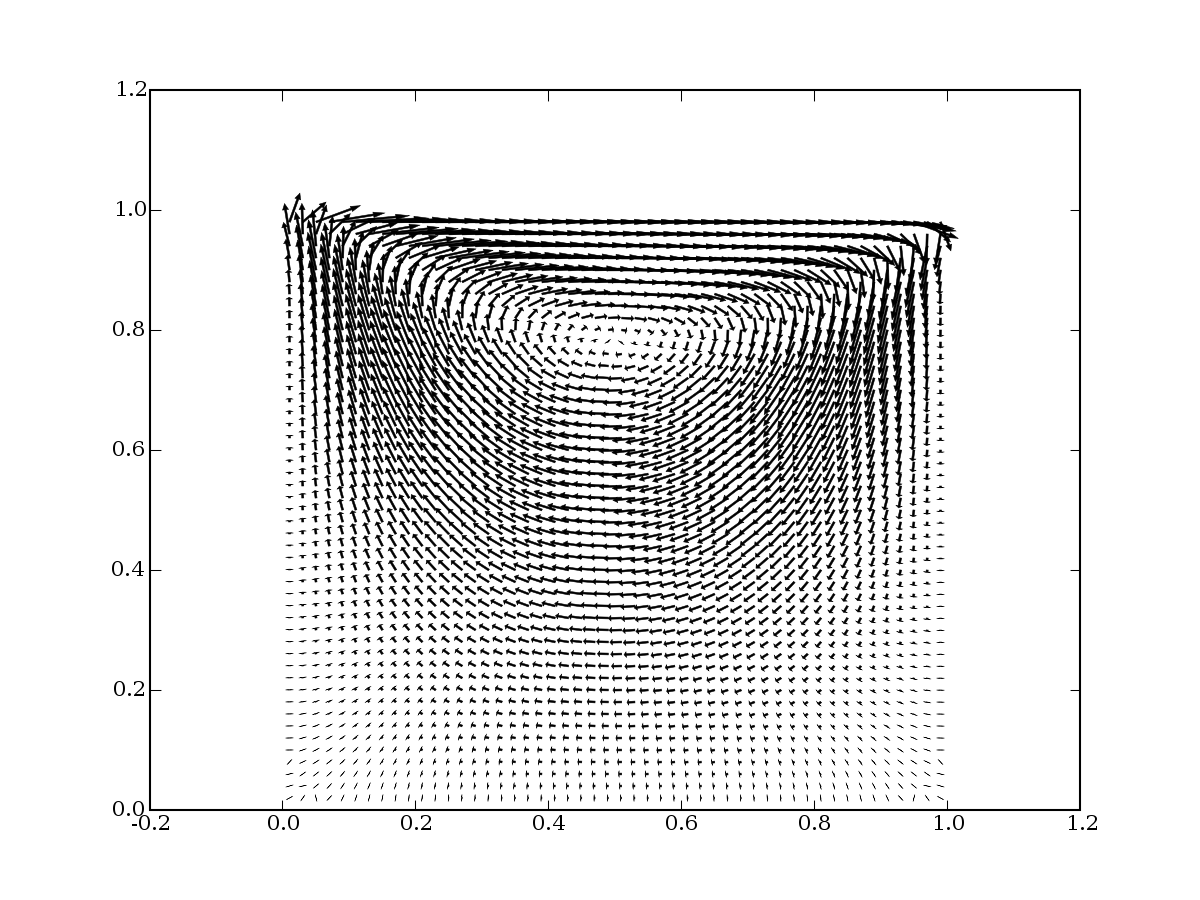
This example is an implementation of a rudimentary Stokes solver on a collocated grid. It solves the Navier-Stokes equation in the viscous limit,

$\nabla \cdot \left( \mu \nabla \vec{u} \right) = \nabla p$

and the continuity equation,

$\nabla \cdot \vec{u} = 0$

where $\vec{u}$ is the fluid velocity, $p$ is the pressure and $\mu$ is the viscosity. The domain in this example is a square cavity of unit dimensions with a moving lid of unit speed. This example uses the SIMPLE algorithm with Rhie-Chow interpolation for collocated grids to solve the pressure-momentum coupling. Some of the details of the algorithm will be highlighted below but a good reference for this material is Ferziger and Peric [27] and Rossow [28]. The solution has a high degree of error close to the corners of the domain for the pressure but does a reasonable job of predicting the velocities away from the boundaries. A number of aspects of FiPy need to be improved to have a first class flow solver. These include, higher order spatial diffusion terms, proper wall boundary conditions, improved mass flux evaluation and extrapolation of cell values to the boundaries using gradients.

In the table below a comparison is made with the Dolfyn open source code on a 100 by 100 grid. The table shows the frequency of values that fall within the given error confidence bands. Dolfyn has the added features described above. When these features are switched off the results of Dolfyn and FiPy are identical.

% frequency of cells	x-velocity error (%)	y-velocity error (%)	pressure error (%)
90	$<0.1$	$< 0.1$	$< 5$
5	0.1 to 0.6	0.1 to 0.3	5 to 11
4	0.6 to 7	0.3 to 4	11 to 35
1	7 to 96	4 to 80	35 to 179
0	$> 96$	$> 80$	$> 179$

To start, some parameters are declared.

>>> from fipy import CellVariable, FaceVariable, Grid2D, DiffusionTerm, Viewer
>>> from fipy.tools import numerix

>>> L = 1.0
>>> N = 50
>>> dL = L / N
>>> viscosity = 1
>>> U = 1.
>>> #0.8 for pressure and 0.5 for velocity are typical relaxation values for SIMPLE
>>> pressureRelaxation = 0.8
>>> velocityRelaxation = 0.5
>>> if __name__ == '__main__':
...     sweeps = 300
... else:
...     sweeps = 5

Build the mesh.

>>> mesh = Grid2D(nx=N, ny=N, dx=dL, dy=dL)

Declare the variables.

>>> pressure = CellVariable(mesh=mesh, name='pressure')
>>> pressureCorrection = CellVariable(mesh=mesh)
>>> xVelocity = CellVariable(mesh=mesh, name='X velocity')
>>> yVelocity = CellVariable(mesh=mesh, name='Y velocity')

The velocity is required as a rank-1 FaceVariable for calculating the mass flux. This is required by the Rhie-Chow correction to avoid pressure/velocity decoupling.

>>> velocity = FaceVariable(mesh=mesh, rank=1)

Build the Stokes equations in the cell centers.

>>> xVelocityEq = DiffusionTerm(coeff=viscosity) - pressure.grad.dot([1., 0.])
>>> yVelocityEq = DiffusionTerm(coeff=viscosity) - pressure.grad.dot([0., 1.])

In this example the SIMPLE algorithm is used to couple the pressure and momentum equations. Let us assume we have solved the discretized momentum equations using a guessed pressure field $p^{\ast}$ to obtain a velocity field $\vec{u}^{\ast}$ . That is $\vec{u}^{\ast}$ is found from

$a_P \vec{u}^{\ast}_P = \sum_f a_A \vec{u}^{\ast}_A - V_P (\nabla p^{\ast})_P$

We would like to somehow correct these initial fields to satisfy both the discretized momentum and continuity equations. We now try to correct these initial fields with a correction such that $\vec{u} = \vec{u}^{\ast} + \vec{u}'$ and $p = p^{\ast} + p'$ , where $\vec{u}$ and $p$ now satisfy the momentum and continuity equations. Substituting the exact solution into the equations we obtain,

$\nabla \cdot \left( \mu \nabla \vec{u}' \right) = \nabla p'$

and

$\nabla \cdot \vec{u}^{\ast} + \nabla \cdot \vec{u}' = 0$

We now use the discretized form of the equations to write the velocity correction in terms of the pressure correction. The discretized form of the above equation results in an equation for $p = p'$ ,

$a_P \vec{u}'_P = \sum_f a_A \vec{u}'_A - V_P (\nabla p')_P$

where notation from Linear Equations is used. The SIMPLE algorithm drops the second term in the above equation to leave,

$\vec{u}'_{P} = - \frac{ V_P (\nabla p')_P }{ a_P }$

By substituting the above expression into the continuity equations we obtain the pressure correction equation,

$\nabla \frac{V_P}{a_P} \cdot \nabla p' = \nabla \cdot \vec{u}^{\ast}$

In the discretized version of the above equation $V_P / a_P$ is approximated at the face by $A_f d_{AP} / (a_P)_f$ . In FiPy the pressure correction equation can be written as,

>>> ap = CellVariable(mesh=mesh, value=1.)
>>> coeff = 1./ ap.arithmeticFaceValue*mesh._faceAreas * mesh._cellDistances
>>> pressureCorrectionEq = DiffusionTerm(coeff=coeff) - velocity.divergence

Above would work good on a staggered grid, however, on a colocated grid as FiPy uses, the term velocity.divergence will cause oscillations in the pressure solution as velocity is a face variable. We can apply the Rhie-Chow correction terms for this. In this an intermediate velocity term $u^\diamond$ is considered which does not contain the pressure corrections:

$\vec{u}^{\diamond}_P = \vec{u}^{\ast}_P + \frac{V_P}{a_P} (\nabla p^{\ast})_P = \sum_f \frac{a_A}{a_P} \vec{u}^{\ast}_A$

This velocity is interpolated at the edges, after which the pressure correction term is added again, but now considered at the edge:

$\vec{u}_f = \frac{1}{2}(\vec{u}^{\diamond}_L + \vec{u}^{\diamond}_R)) - \left(\frac{V}{a_P}\right)_{\mathrm{avg\ L,R}} (\nabla p^{\ast}_f)$

where $\left(\frac{V}{a_P}\right)_{\mathrm{avg\ L,R}}$ is assumed a good approximation at the edge. Here L and R denote the two cells adjacent to the face. Expanding the not calculated terms we arrive at

$\vec{u}_f = \frac{1}{2}(\vec{u}^{\ast}_L + \vec{u}^{\ast}_R)) + \frac{1}{2}\left(\frac{V}{a_P}\right)_{\mathrm{avg\ L,R}} (\nabla p^{\ast}_L+ \nabla p^{\ast}_R) - \left(\frac{V}{a_P}\right)_{\mathrm{avg\ L,R}} (\nabla p^{\ast}_f)$

where we have replaced the coefficients of the cell pressure gradients by an averaged value over the edge. This formula has the consequence that the velocity on a face depends not only on the pressure of the adjacent cells, but also on the cells further away, which removes the unphysical pressure oscillations. We start by introducing needed terms

>>> from fipy.variables.faceGradVariable import _FaceGradVariable
>>> volume = CellVariable(mesh=mesh, value=mesh.cellVolumes, name='Volume')
>>> contrvolume=volume.arithmeticFaceValue

And set up the velocity with this formula in the SIMPLE loop. Now, set up the no-slip boundary conditions

>>> xVelocity.constrain(0., mesh.facesRight | mesh.facesLeft | mesh.facesBottom)
>>> xVelocity.constrain(U, mesh.facesTop)
>>> yVelocity.constrain(0., mesh.exteriorFaces)
>>> X, Y = mesh.faceCenters
>>> pressureCorrection.constrain(0., mesh.facesLeft & (Y < dL))

Set up the viewers,

>>> if __name__ == '__main__':
...     viewer = Viewer(vars=(pressure, xVelocity, yVelocity, velocity),
...                xmin=0., xmax=1., ymin=0., ymax=1., colorbar='vertical', scale=5)

Below, we iterate for a set number of sweeps. We use the sweep() method instead of solve() because we require the residual for output. We also use the cacheMatrix(), matrix, cacheRHSvector() and RHSvector because both the matrix and RHS vector are required by the SIMPLE algorithm. Additionally, the sweep() method is passed an underRelaxation factor to relax the solution. This argument cannot be passed to solve().

>>> from builtins import range
>>> for sweep in range(sweeps):
...
...     ## solve the Stokes equations to get starred values
...     xVelocityEq.cacheMatrix()
...     xres = xVelocityEq.sweep(var=xVelocity,
...                              underRelaxation=velocityRelaxation)
...     xmat = xVelocityEq.matrix
...
...     yres = yVelocityEq.sweep(var=yVelocity,
...                              underRelaxation=velocityRelaxation)
...
...     ## update the ap coefficient from the matrix diagonal
...     ap[:] = -numerix.asarray(xmat.takeDiagonal())
...
...     ## update the face velocities based on starred values with the
...     ## Rhie-Chow correction.
...     ## cell pressure gradient
...     presgrad = pressure.grad
...     ## face pressure gradient
...     facepresgrad = _FaceGradVariable(pressure)
...
...     velocity[0] = xVelocity.arithmeticFaceValue \
...          + contrvolume / ap.arithmeticFaceValue * \
...            (presgrad[0].arithmeticFaceValue-facepresgrad[0])
...     velocity[1] = yVelocity.arithmeticFaceValue \
...          + contrvolume / ap.arithmeticFaceValue * \
...            (presgrad[1].arithmeticFaceValue-facepresgrad[1])
...     velocity[..., mesh.exteriorFaces.value] = 0.
...     velocity[0, mesh.facesTop.value] = U
...
...     ## solve the pressure correction equation
...     pressureCorrectionEq.cacheRHSvector()
...     ## left bottom point must remain at pressure 0, so no correction
...     pres = pressureCorrectionEq.sweep(var=pressureCorrection)
...     rhs = pressureCorrectionEq.RHSvector
...
...     ## update the pressure using the corrected value
...     pressure.setValue(pressure + pressureRelaxation * pressureCorrection )
...     ## update the velocity using the corrected pressure
...     xVelocity.setValue(xVelocity - pressureCorrection.grad[0] / \
...                                                ap * mesh.cellVolumes)
...     yVelocity.setValue(yVelocity - pressureCorrection.grad[1] / \
...                                                ap * mesh.cellVolumes)
...
...     if __name__ == '__main__':
...         if sweep%10 == 0:
...             print('sweep:', sweep, ', x residual:', xres, \
...                                  ', y residual', yres, \
...                                  ', p residual:', pres, \
...                                  ', continuity:', max(abs(rhs)))
...
...             viewer.plot()

Test values in the last cell.

>>> print(numerix.allclose(pressure.globalValue[..., -1], 162.790867927)) 
1
>>> print(numerix.allclose(xVelocity.globalValue[..., -1], 0.265072740929)) 
1
>>> print(numerix.allclose(yVelocity.globalValue[..., -1], -0.150290488304)) 
1

Last updated on Jun 27, 2023. Created using Sphinx 6.2.1.