-
Citation: S.M. Foiles, M.I. Baskes, and M.S. Daw (1986), "Embedded-atom-method functions for the fcc metals Cu, Ag, Au, Ni, Pd, Pt, and their alloys", Physical Review B 33(12), 7983-7991. DOI: 10.1103/physrevb.33.7983.Abstract: A consistent set of embedding functions and pair interactions for use with the embedded-atom method [M.S. Daw and M. I. Baskes, Phys. Rev. B 29, 6443 (1984)] have been determined empirically to describe the fcc metals Cu, Ag, Au, Ni, Pd, and Pt as well as alloys containing these metals. The functions are determined empirically by fitting to the sublimation energy, equilibrium lattice constant, elastic constants, and vacancy-formation energies of the pure metals and the heats of solution of the binary alloys. The validity of the functions is tested by computing a wide range of properties: the formation volume and migration energy of vacancies, the formation energy, formation volume, and migration energy of divacancies and self-interstitials, the surface energy and geometries of the low-index surfaces of the pure metals, and the segregation energy of substitutional impurities to (100) surfaces.
Related Models: -
LAMMPS pair_style eam (1986--Foiles-S-M--Ni--LAMMPS--ipr1)See Computed Properties
Notes: This file was taken from the August 22, 2018 LAMMPS distribution.
File(s): -
OpenKIM (MO_580571659842)See Computed Properties
Notes: Listing found at https://openkim.org. This KIM potential is based on the same files as 1986--Foiles-S-M--Ni--LAMMPS--ipr1.
Link(s):
Implementation Information
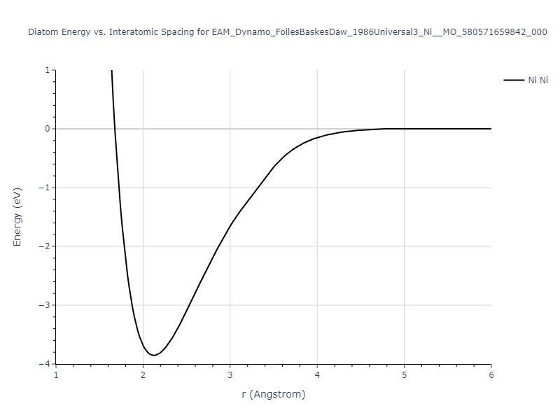
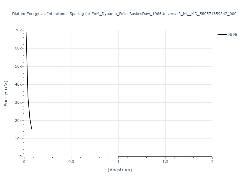
Diatom Energy vs. Interatomic Spacing
Plots of the potential energy vs interatomic spacing, r, are shown below for all diatom sets associated with the interatomic potential. This calculation provides insights into the functional form of the potential's two-body interactions. A system consisting of only two atoms is created, and the potential energy is evaluated for the atoms separated by 0.02 Å <= r <= 6.0> Å in intervals of 0.02 Å. Two plots are shown: one for the "standard" interaction distance range, and one for small values of r. The small r plot is useful for determining whether the potential is suitable for radiation studies.
The calculation method used is available as the iprPy diatom_scan calculation method.
Clicking on the image of a plot will open an interactive version of it in a new tab. The underlying data for the plots can be downloaded by clicking on the links above each plot.
Notes and Disclaimers:
- These values are meant to be guidelines for comparing potentials, not the absolute values for any potential's properties. Values listed here may change if the calculation methods are updated due to improvements/corrections. Variations in the values may occur for variations in calculation methods, simulation software and implementations of the interatomic potentials.
- As this calculation only involves two atoms, it neglects any multi-body interactions that may be important in molecules, liquids and crystals.
- NIST disclaimer
Version Information:
- 2019-11-14. Maximum value range on the shortrange plots are now limited to "expected" levels as details are otherwise lost.
- 2019-08-07. Plots added.
Click on plot to load interactive version
Click on plot to load interactive version
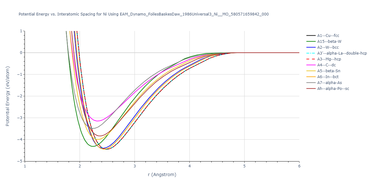
Cohesive Energy vs. Interatomic Spacing
Plots of potential energy vs interatomic spacing, r, are shown below for a number of crystal structures. The structures are generated based on the ideal atomic positions and b/a and c/a lattice parameter ratios for a given crystal prototype. The size of the system is then uniformly scaled, and the energy calculated without relaxing the system. To obtain these plots, values of r are evaluated every 0.02 Å up to 6 Å.
The calculation method used is available as the iprPy E_vs_r_scan calculation method.
Clicking on the image of a plot will open an interactive version of it in a new tab. The underlying data for the plots can be downloaded by clicking on the links above each plot.
Notes and Disclaimers:
- These values are meant to be guidelines for comparing potentials, not the absolute values for any potential's properties. Values listed here may change if the calculation methods are updated due to improvements/corrections. Variations in the values may occur for variations in calculation methods, simulation software and implementations of the interatomic potentials.
- The minima identified by this calculation do not guarantee that the associated crystal structures will be stable since no relaxation is performed.
- NIST disclaimer
Version Information:
- 2020-12-18. Descriptions, tables and plots updated to reflect that the energy values are the measuredper atom potential energy rather than cohesive energy as some potentials have non-zero isolated atom energies.
- 2019-02-04. Values regenerated with even r spacings of 0.02 Å, and now include values less than 2 Å when possible. Updated calculation method and parameters enhance compatibility with more potential styles.
- 2019-04-26. Results for hcp, double hcp, α-As and L10 prototypes regenerated from different unit cell representations. Only α-As results show noticable (>1e-5 eV) difference due to using a different coordinate for Wykoff site c position.
- 2018-06-13. Values for MEAM potentials corrected. Dynamic versions of the plots moved to separate pages to improve page loading. Cosmetic changes to how data is shown and updates to the documentation.
- 2017-01-11. Replaced png pictures with interactive Bokeh plots. Data regenerated with 200 values of r instead of 300.
- 2016-09-28. Plots for binary structures added. Data and plots for elemental structures regenerated. Data values match the values of the previous version. Data table formatting slightly changed to increase precision and ensure spaces between large values. Composition added to plot title and structure names made longer.
- 2016-04-07. Plots for elemental structures added.
Crystal Structure Predictions
Computed lattice constants and cohesive/potential energies are displayed for a variety of crystal structures. The values displayed here are obtained using the following process.
- Initial crystal structure guesses are taken from:
- The iprPy E_vs_r_scan calculation results (shown above) by identifying all energy minima along the measured curves for a given crystal prototype + composition.
- Structures in the Materials Project and OQMD DFT databases.
- All initial guesses are relaxed using three independent methods using a 10x10x10 supercell:
- "box": The system's lattice constants are adjusted to zero pressure without internal relaxations using the iprPy relax_box calculation with a strainrange of 1e-6.
- "static": The system's lattice and atomic positions are statically relaxed using the iprPy relax_static calculation with a minimization force tolerance of 1e-10 eV/Angstrom.
- "dynamic": The system's lattice and atomic positions are dynamically relaxed for 10000 timesteps of 0.01 ps using the iprPy relax_dynamic calculation with an nph integration plus Langevin thermostat. The final configuration is then used as input in running an iprPy relax_static calculation with a minimization force tolerance of 1e-10 eV/Angstrom.
- The relaxed structures obtained from #2 are then evaluated using the spglib package to identify an ideal crystal unit cell based on the results.
- The space group information of the ideal unit cells is compared to the space group information of the corresponding reference structures to identify which structures transformed upon relaxation. The structures that did not transform to a different structure are listed in the table(s) below. The "method" field indicates the most rigorous relaxation method where the structure did not transform. The space group information is also used to match the DFT reference structures to the used prototype, where possible.
- The cohesive energy, Ecoh, is calculated from the measured potential energy per atom, Epot$, by subtracting the isolated energy averaged across all atoms in the unit cell. The isolated atom energies of each species model is obtained either by evaluating a single atom atomic configuration, or by identifying the first energy plateau from the diatom scan calculations for r > 2 Å.
The calculation methods used are implemented into iprPy as the following calculation styles
Notes and Disclaimers:
- These values are meant to be guidelines for comparing potentials, not the absolute values for any potential's properties. Values listed here may change if the calculation methods are updated due to improvements/corrections. Variations in the values may occur for variations in calculation methods, simulation software and implementations of the interatomic potentials.
- The presence of any structures in this list does not guarantee that those structures are stable. Also, the lowest energy structure may not be included in this list.
- Multiple values for the same crystal structure but different lattice constants are possible. This is because multiple energy minima are possible for a given structure and interatomic potential. Having multiple energy minima for a structure does not necessarily make the potential "bad" as unwanted configurations may be unstable or correspond to conditions that may not be relevant to the problem of interest (eg. very high strains).
- NIST disclaimer
Version Information:
- 2025-07-02. All "mp-" reference structure calculations were re-relaxed using the updated Materials Project database rather than the original database structures. Also, a bug was fixed that caused the "static" relaxations to occasionally throw unnecessary errors. This was fixed and all affected calculations were reset and performed again.
- 2022-05-27. The "box" method results have all been redone with an updated methodology more suited for non-orthogonal systems.
- 2020-12-18. Cohesive energies have been corrected by making them relative to the energies of the isolated atoms. The previous cohesive energy values are now listed as the potential energies.
- 2019-06-07. Structures with positive or near zero cohesive energies removed from the display tables. All values still present in the raw data files.
- 2019-04-26. Calculations now computed for each implementation. Results for hcp, double hcp, α-As and L10 prototypes regenerated from different unit cell representations.
- 2018-06-14. Methodology completely changed affecting how the information is displayed. Calculations involving MEAM potentials corrected.
- 2016-09-28. Values for simple compounds added. All identified energy minima for each structure are listed. The existing elemental data was regenerated. Most values are consistent with before, but some differences have been noted. Specifically, variations are seen with some values for potentials where the elastic constants don't vary smoothly near the equilibrium state. Additionally, the inclusion of some high-energy structures has changed based on new criteria for identifying when structures have relaxed to another structure.
- 2016-04-07. Values for elemental crystal structures added. Only values for the global energy minimum of each unique structure given.
Download raw data (including filtered results)
Reference structure matches:
A1--Cu--fcc = mp-23, oqmd-676148, oqmd-1214550
A15--beta-W = oqmd-1214995, oqmd-1280360
A2--W--bcc = mp-1008728, oqmd-22516, oqmd-1215173
A3'--alpha-La--double-hcp = oqmd-1215441
A3--Mg--hcp = mp-10257, oqmd-677944, oqmd-1215351
A4--C--dc = oqmd-1215530
A5--beta-Sn = oqmd-1215619
A6--In--bct = oqmd-1215708
| prototype | method | Ecoh (eV/atom) | Epot (eV/atom) | a0 (Å) | b0 (Å) | c0 (Å) | α (degrees) | β (degrees) | γ (degrees) |
|---|---|---|---|---|---|---|---|---|---|
| A1--Cu--fcc | dynamic | -4.45 | -4.45 | 3.52 | 3.52 | 3.52 | 90.0 | 90.0 | 90.0 |
| A3'--alpha-La--double-hcp | dynamic | -4.4488 | -4.4488 | 2.4892 | 2.4892 | 8.1223 | 90.0 | 90.0 | 120.0 |
| oqmd-1216067 | dynamic | -4.4484 | -4.4484 | 2.4892 | 2.4892 | 18.2701 | 90.0 | 90.0 | 120.0 |
| A3--Mg--hcp | dynamic | -4.4476 | -4.4476 | 2.4893 | 2.4893 | 4.0578 | 90.0 | 90.0 | 120.0 |
| oqmd-1215262 | box | -4.447 | -4.447 | 2.4802 | 4.3272 | 4.0584 | 90.0 | 90.0 | 90.0 |
| A2--W--bcc | static | -4.4018 | -4.4018 | 2.7989 | 2.7989 | 2.7989 | 90.0 | 90.0 | 90.0 |
| oqmd-1214906 | dynamic | -4.3651 | -4.3651 | 6.0796 | 6.0796 | 6.0796 | 90.0 | 90.0 | 90.0 |
| oqmd-1214906 | box | -4.3649 | -4.3649 | 6.0771 | 6.0771 | 6.0771 | 90.0 | 90.0 | 90.0 |
| oqmd-1214817 | dynamic | -4.3509 | -4.3509 | 8.6575 | 8.6575 | 8.6575 | 90.0 | 90.0 | 90.0 |
| oqmd-1214817 | box | -4.3497 | -4.3497 | 8.6566 | 8.6566 | 8.6566 | 90.0 | 90.0 | 90.0 |
| A15--beta-W | dynamic | -4.319 | -4.319 | 4.4801 | 4.4801 | 4.4801 | 90.0 | 90.0 | 90.0 |
| oqmd-1215084 | box | -4.2315 | -4.2315 | 2.5014 | 4.1887 | 8.9141 | 90.0 | 90.0 | 90.0 |
| oqmd-1214728 | box | -4.1264 | -4.1264 | 2.4203 | 2.4203 | 8.4279 | 90.0 | 90.0 | 90.0 |
| A5--beta-Sn | static | -4.0109 | -4.0109 | 4.5484 | 4.5484 | 2.3961 | 90.0 | 90.0 | 90.0 |
| mp-1014111 | dynamic | -3.9699 | -3.9699 | 2.4771 | 2.4771 | 13.4929 | 90.0 | 90.0 | 120.0 |
| mp-1014111 | static | -3.9699 | -3.9699 | 2.4771 | 2.4771 | 13.4964 | 90.0 | 90.0 | 120.0 |
| Ah--alpha-Po--sc | static | -3.837 | -3.837 | 2.3658 | 2.3658 | 2.3658 | 90.0 | 90.0 | 90.0 |
| A7--alpha-As | box | -3.4678 | -3.4678 | 3.2304 | 3.2304 | 10.1031 | 90.0 | 90.0 | 120.0 |
| oqmd-1215975 | box | -3.4559 | -3.4559 | 4.0166 | 4.0166 | 4.4694 | 90.0 | 90.0 | 120.0 |
| A4--C--dc | static | -3.1503 | -3.1503 | 5.3751 | 5.3751 | 5.3751 | 90.0 | 90.0 | 90.0 |
Elastic Constants Predictions
Static elastic constants are displayed for the unique structures identified in Crystal Structure Predictions above. The values displayed here are obtained by measuring the change in virial stresses due to applying small strains to the relaxed crystals. The initial structure and the strained states are all relaxed using force minimization.
The calculation method used is available as the iprPy elastic_constants_static calculation method.
Notes and Disclaimers:
- These values are meant to be guidelines for comparing potentials, not the absolute values for any potential's properties. Values listed here may change if the calculation methods are updated due to improvements/corrections. Variations in the values may occur for variations in calculation methods, simulation software and implementations of the interatomic potentials.
- The presence of any structures in this list does not guarantee that those structures are stable.
- The elastic constants have been computed for a variety of strains, and in some cases for slightly different lattice constant values. The static nature of this calculation can give poor predictions if the evaluated states straddle a functional discontinuity in the potential's third derivative. Be sure to compare the elastic constants for the different strains (positive and negative).
- NIST disclaimer
Version Information:
- 2019-08-07. Data added.
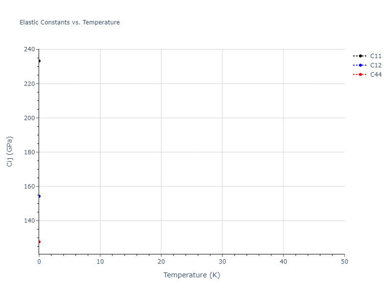
| 233.273 | 154.287 | 154.287 | 0.000 | 0.000 | 0.000 |
| 154.287 | 233.273 | 154.287 | 0.000 | 0.000 | 0.000 |
| 154.287 | 154.287 | 233.273 | -0.000 | 0.000 | 0.000 |
| -0.000 | 0.000 | 0.000 | 127.637 | 0.000 | -0.000 |
| 0.000 | -0.000 | 0.000 | 0.000 | 127.637 | -0.000 |
| 0.000 | 0.000 | -0.000 | -0.000 | -0.000 | 127.637 |
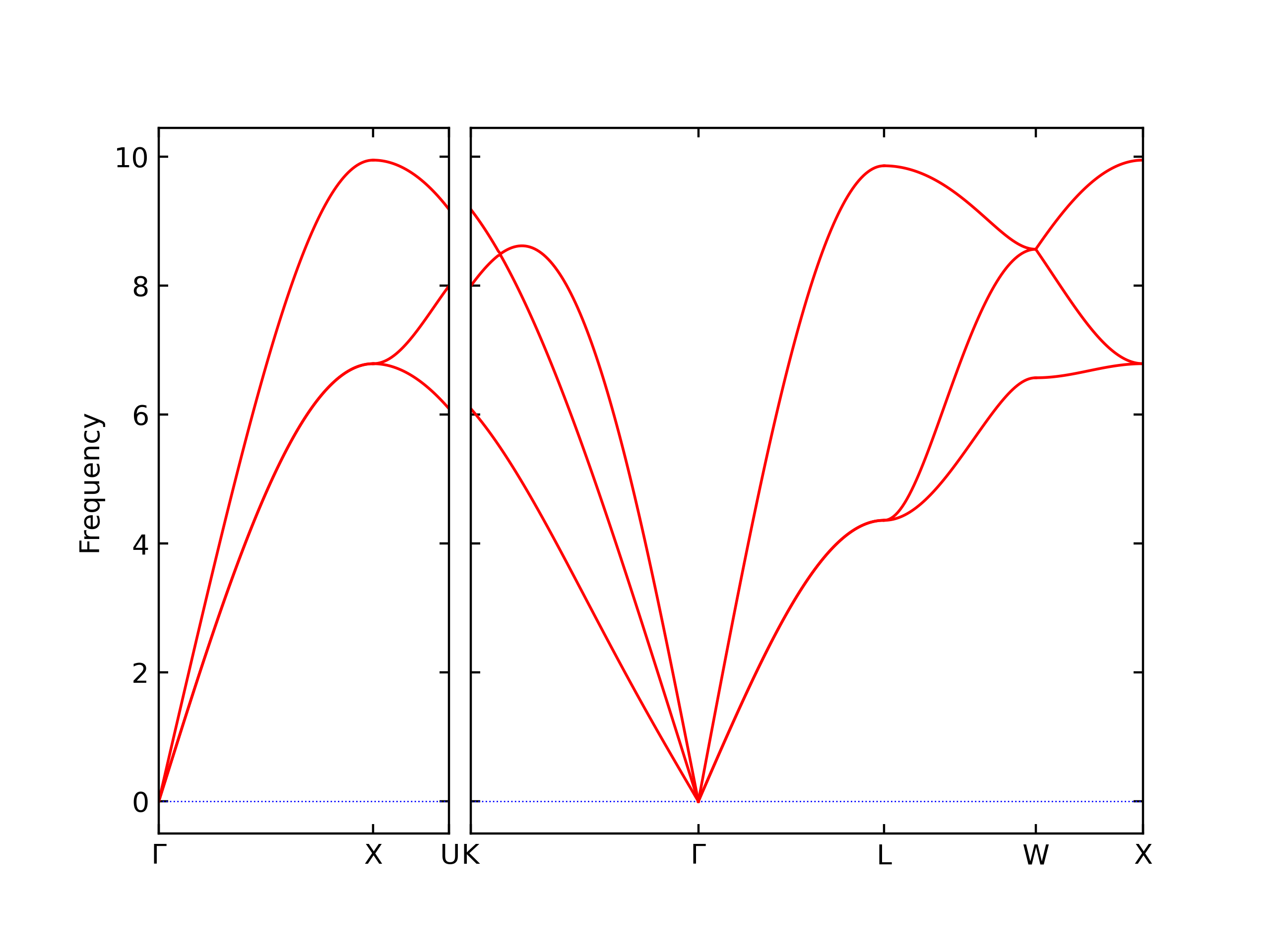
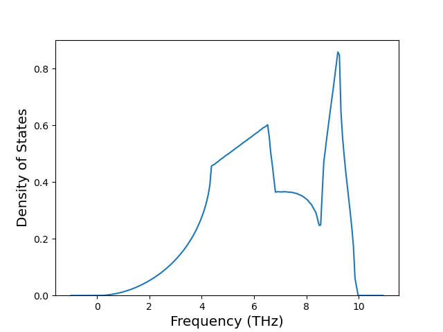
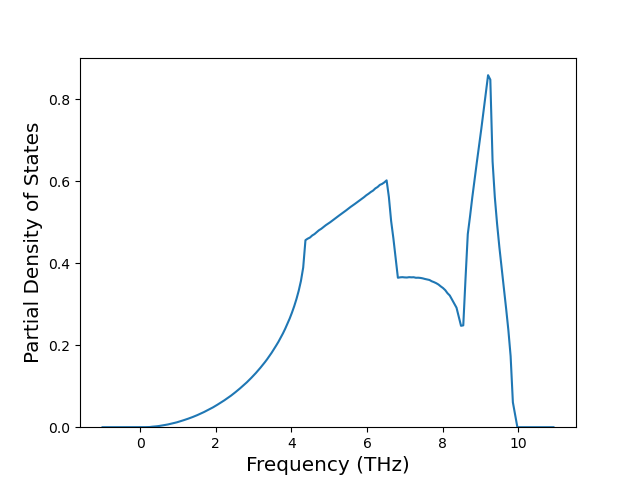
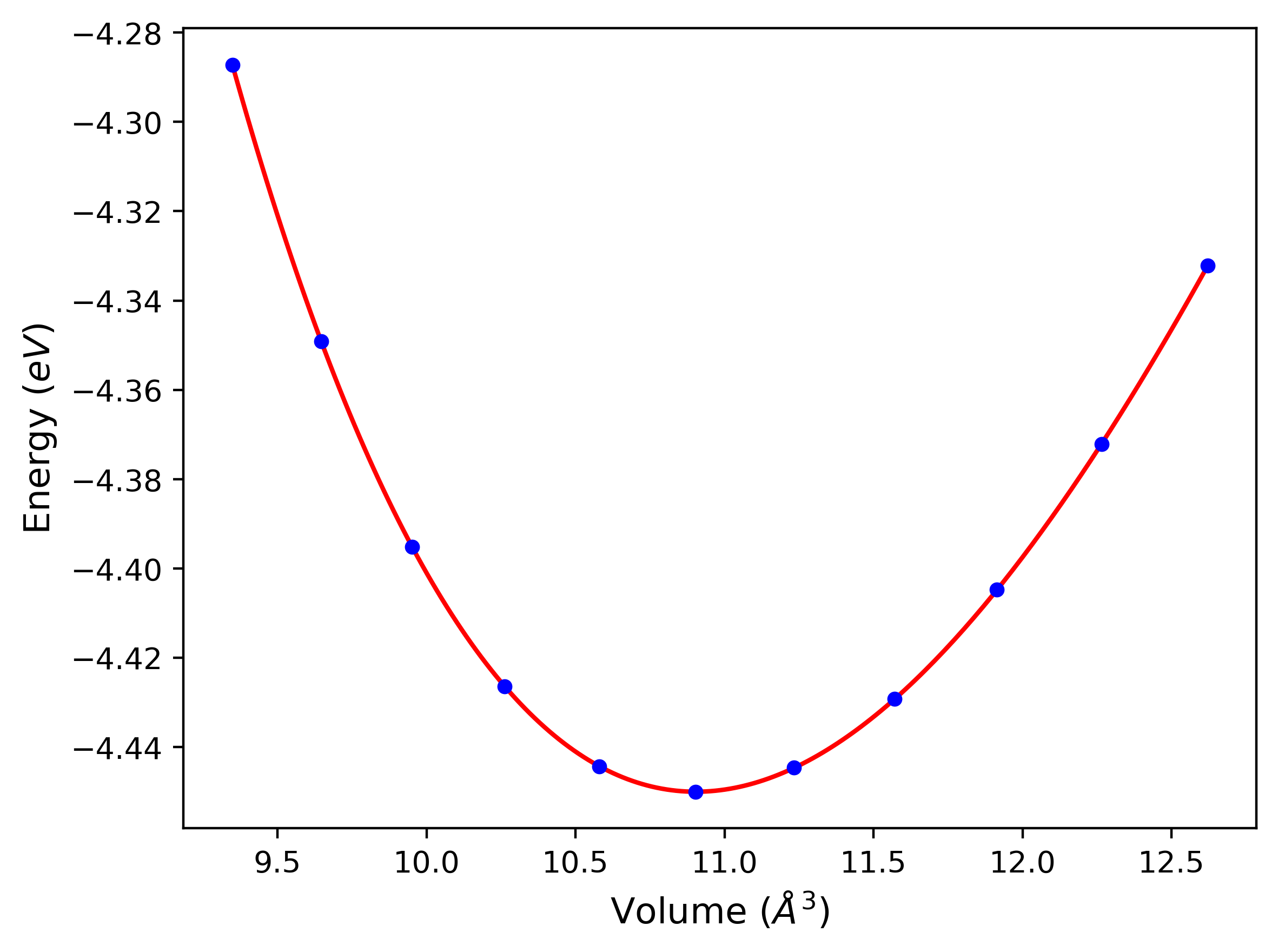
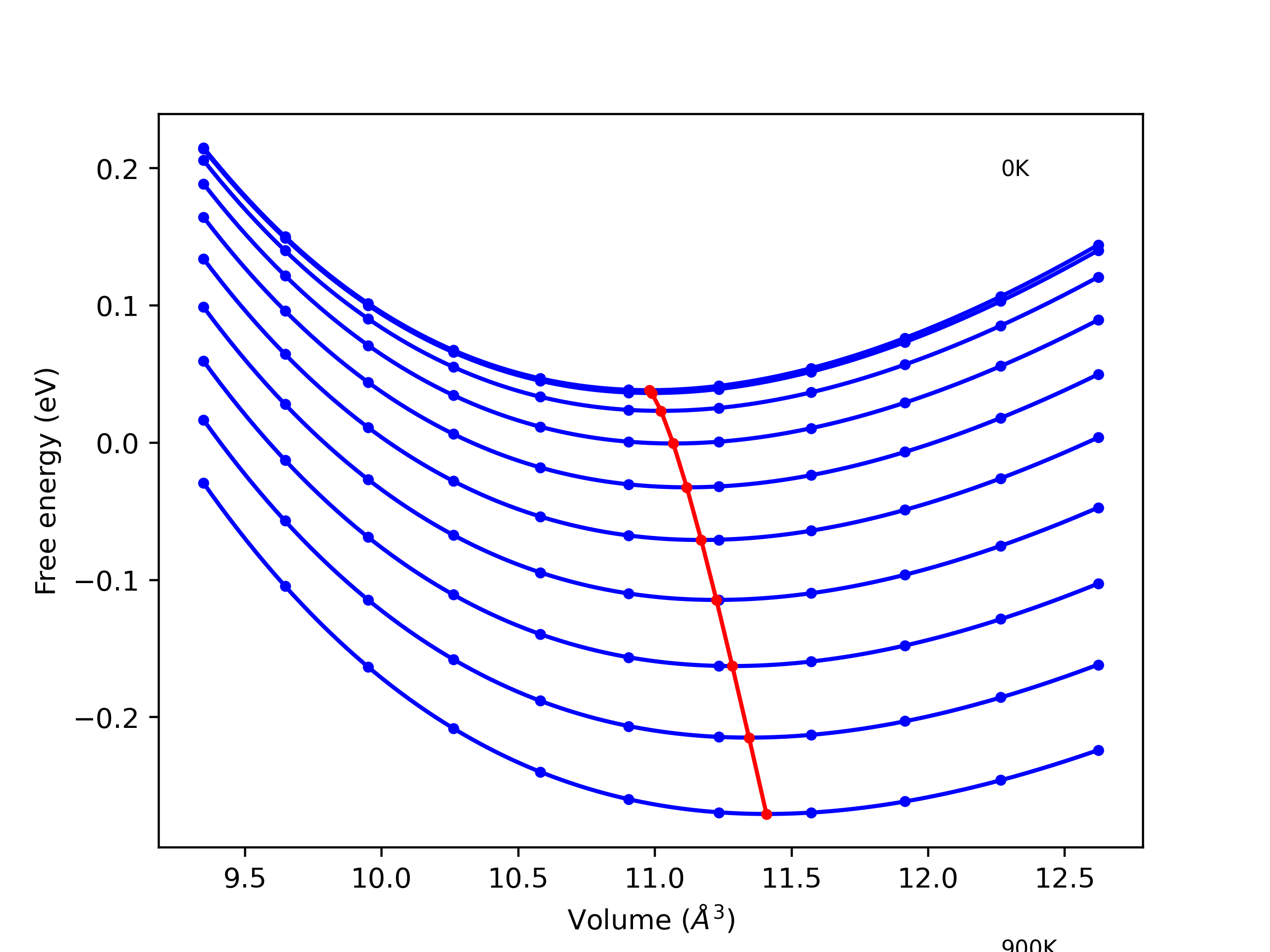
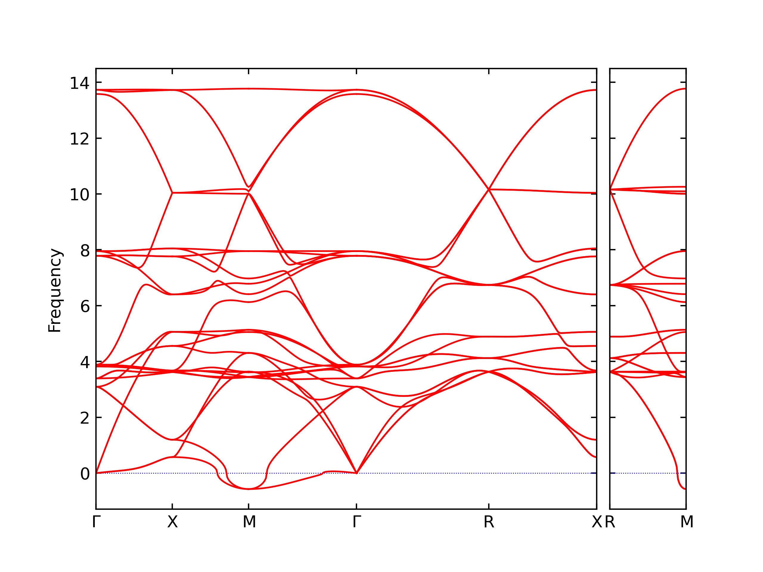
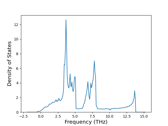
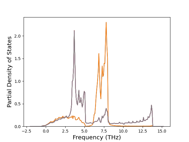
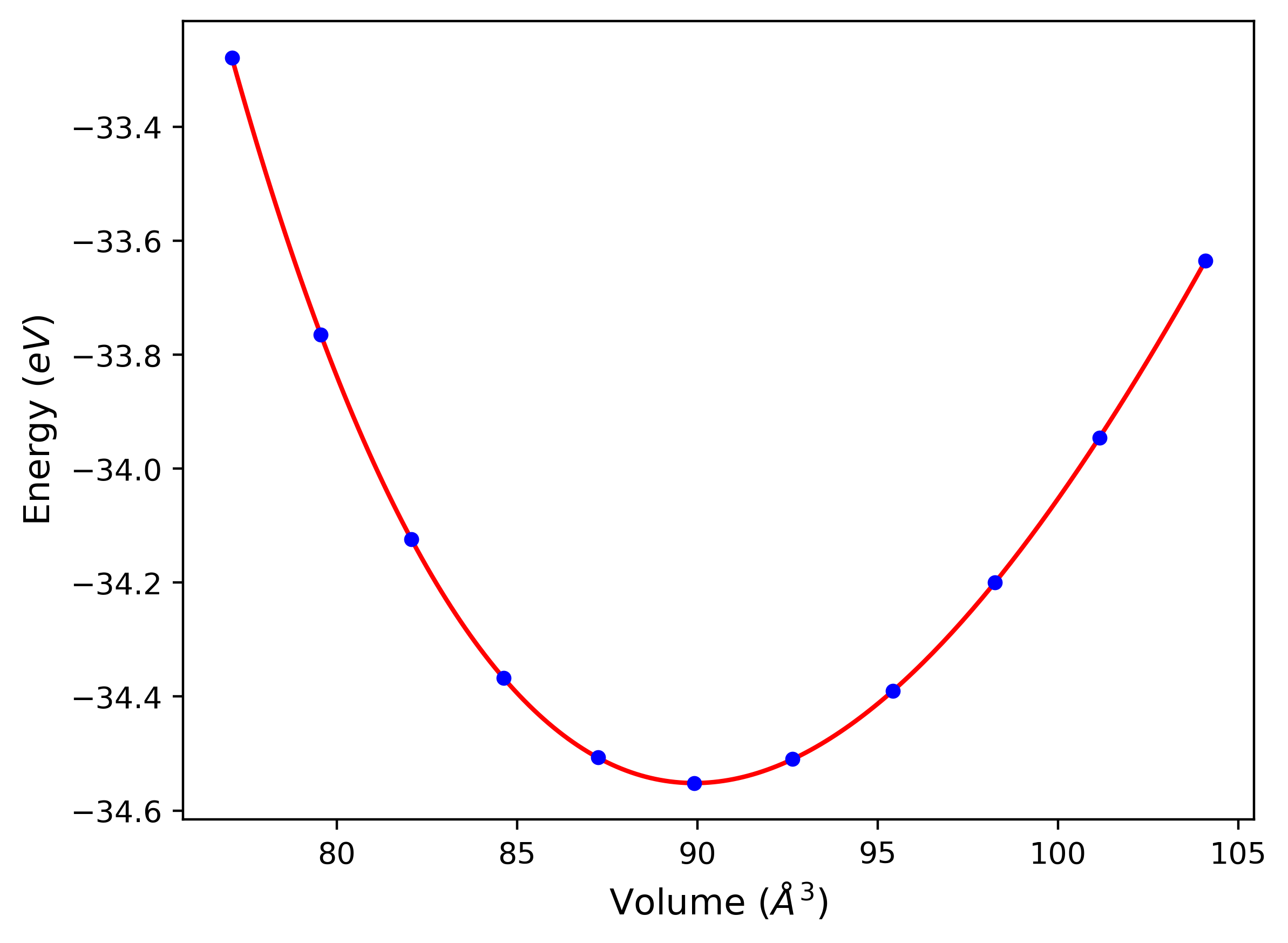
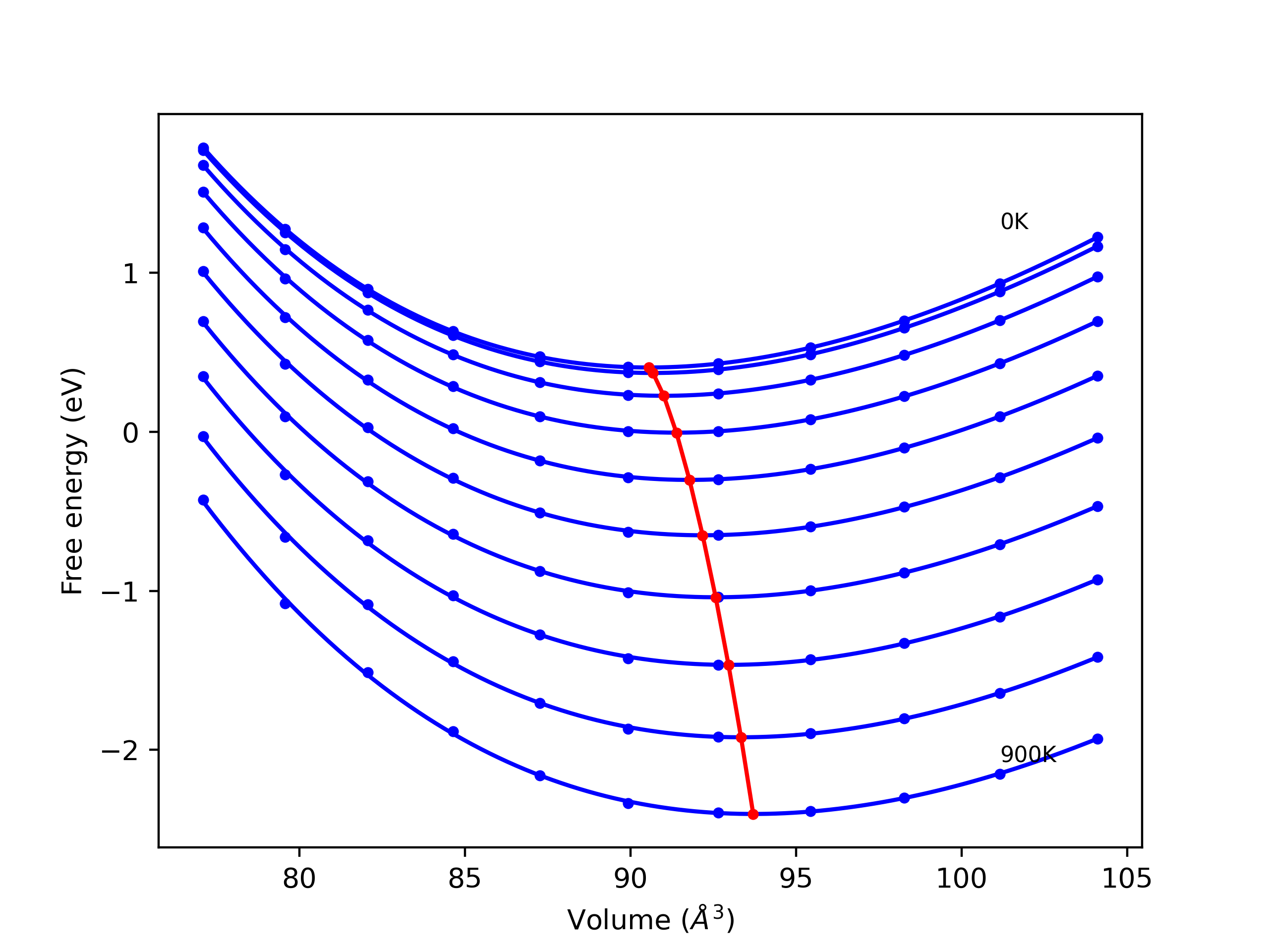
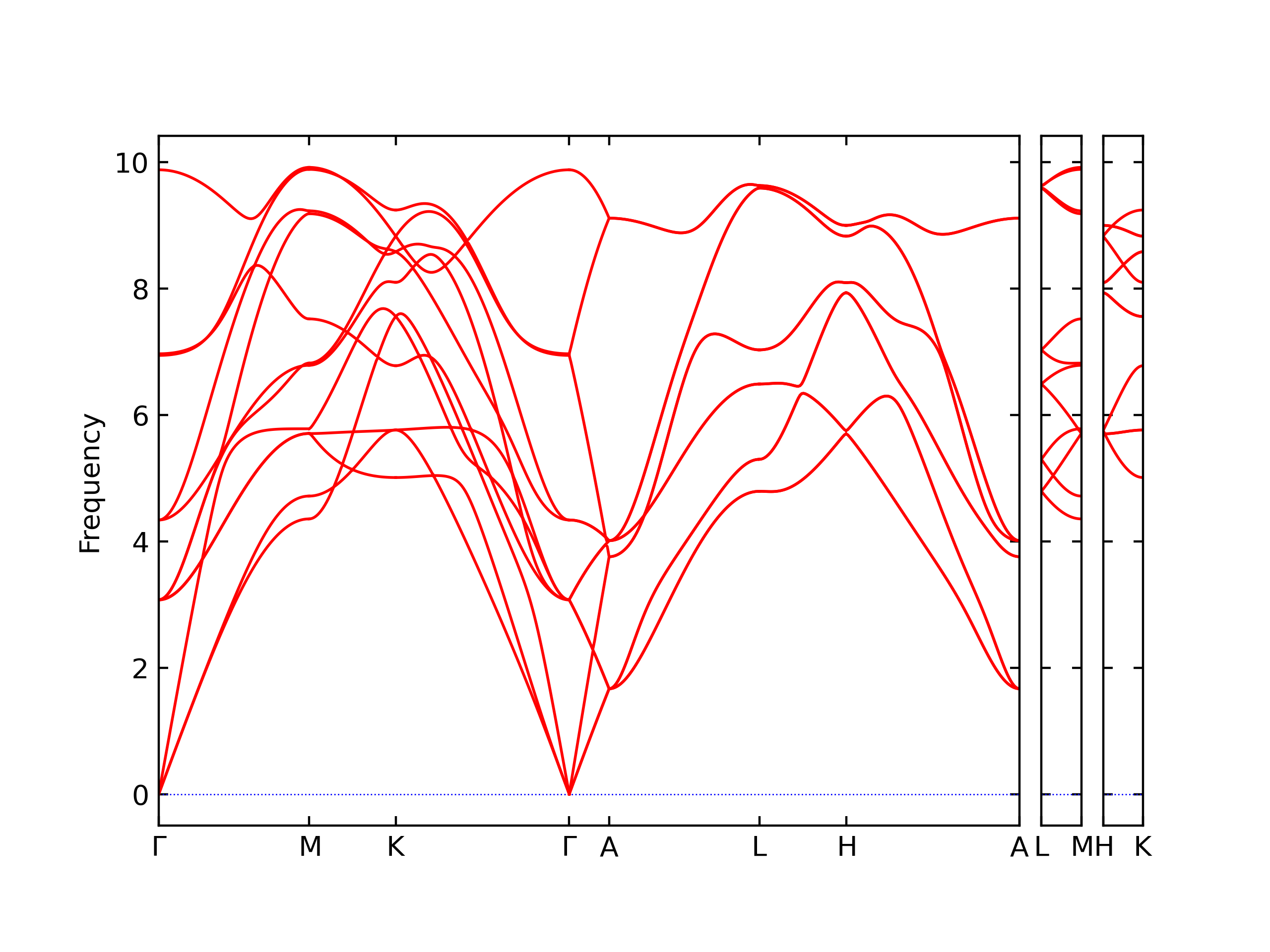
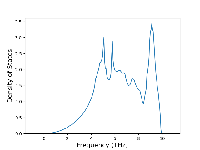
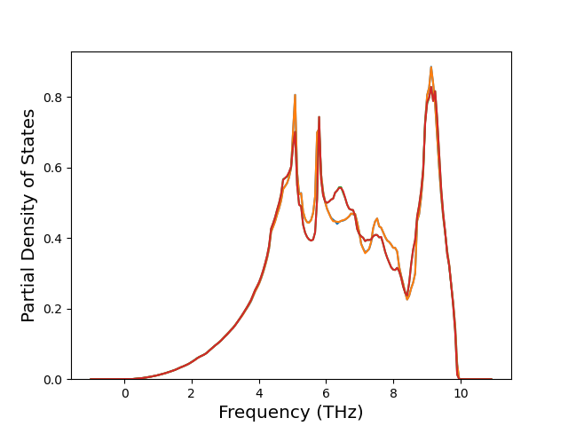
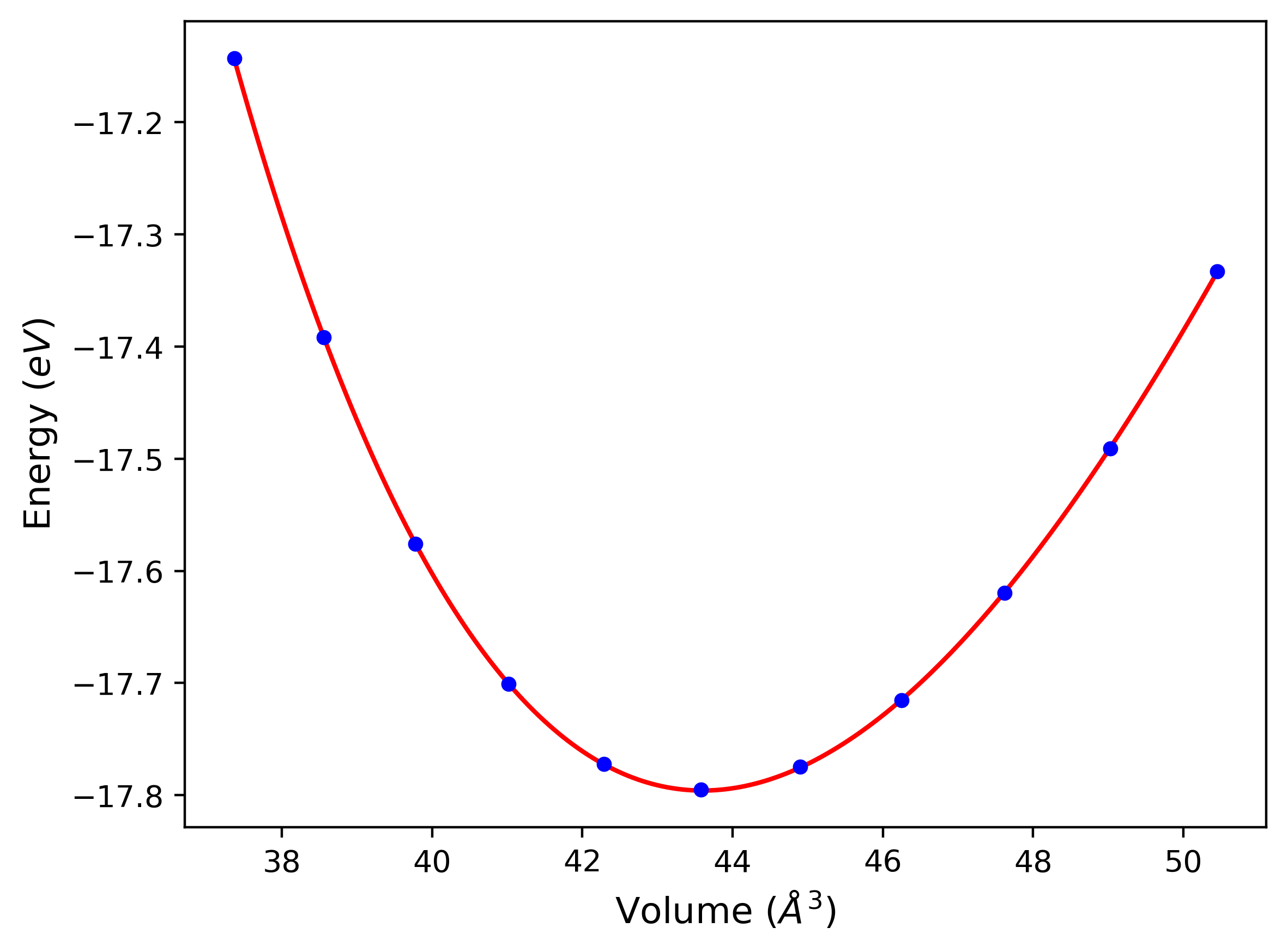
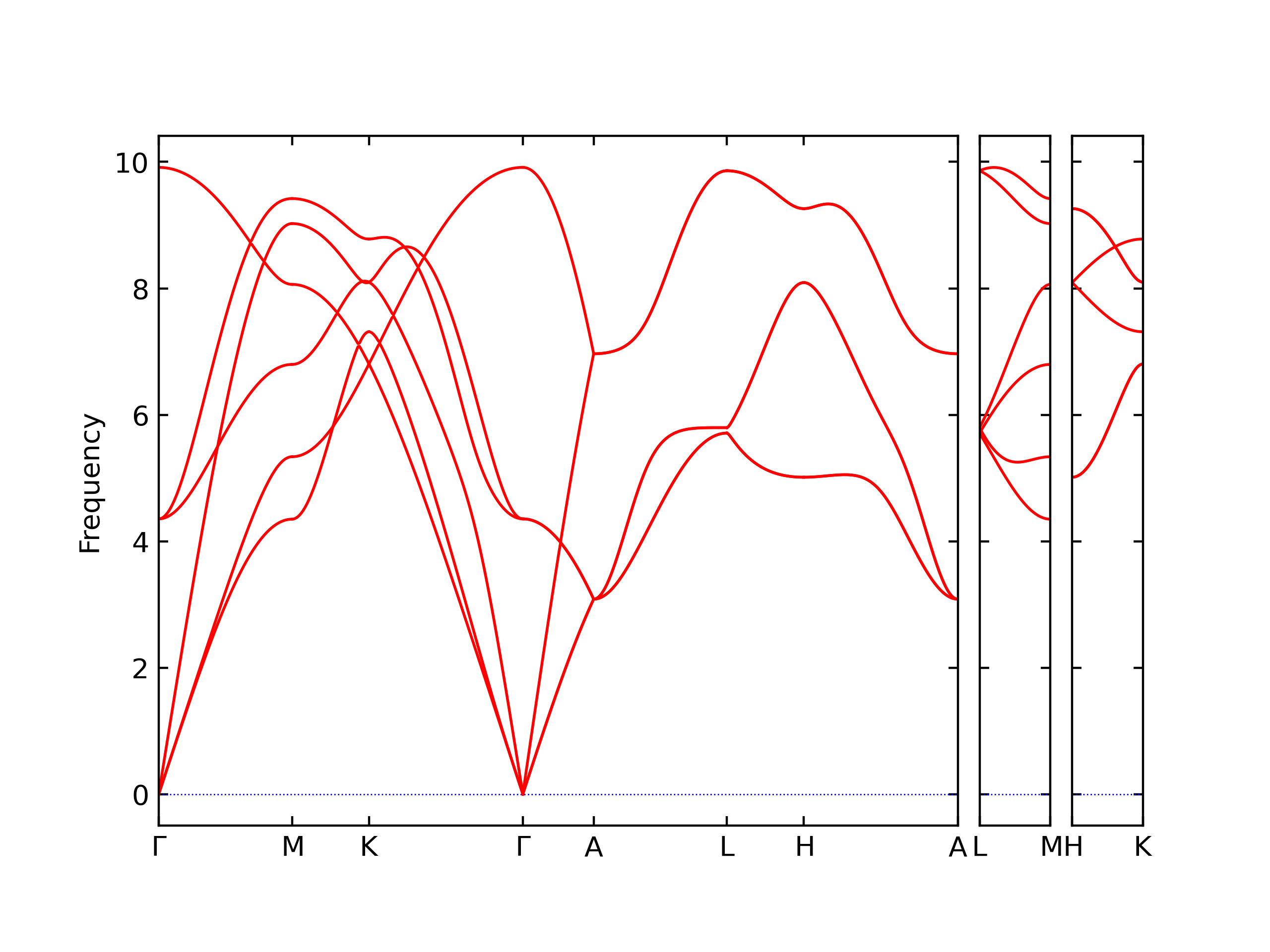
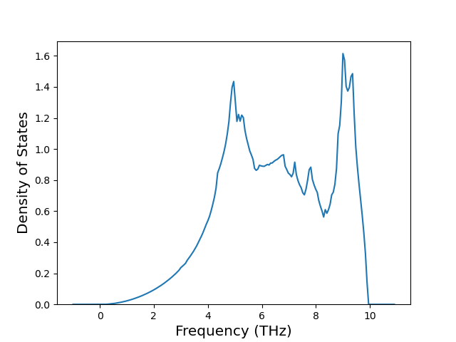
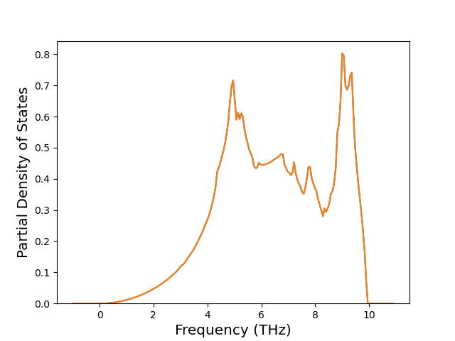
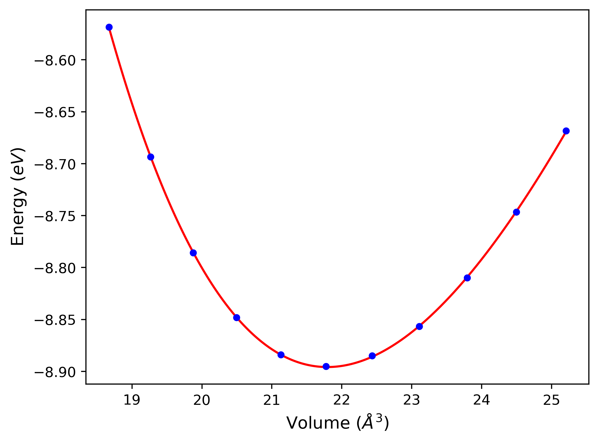
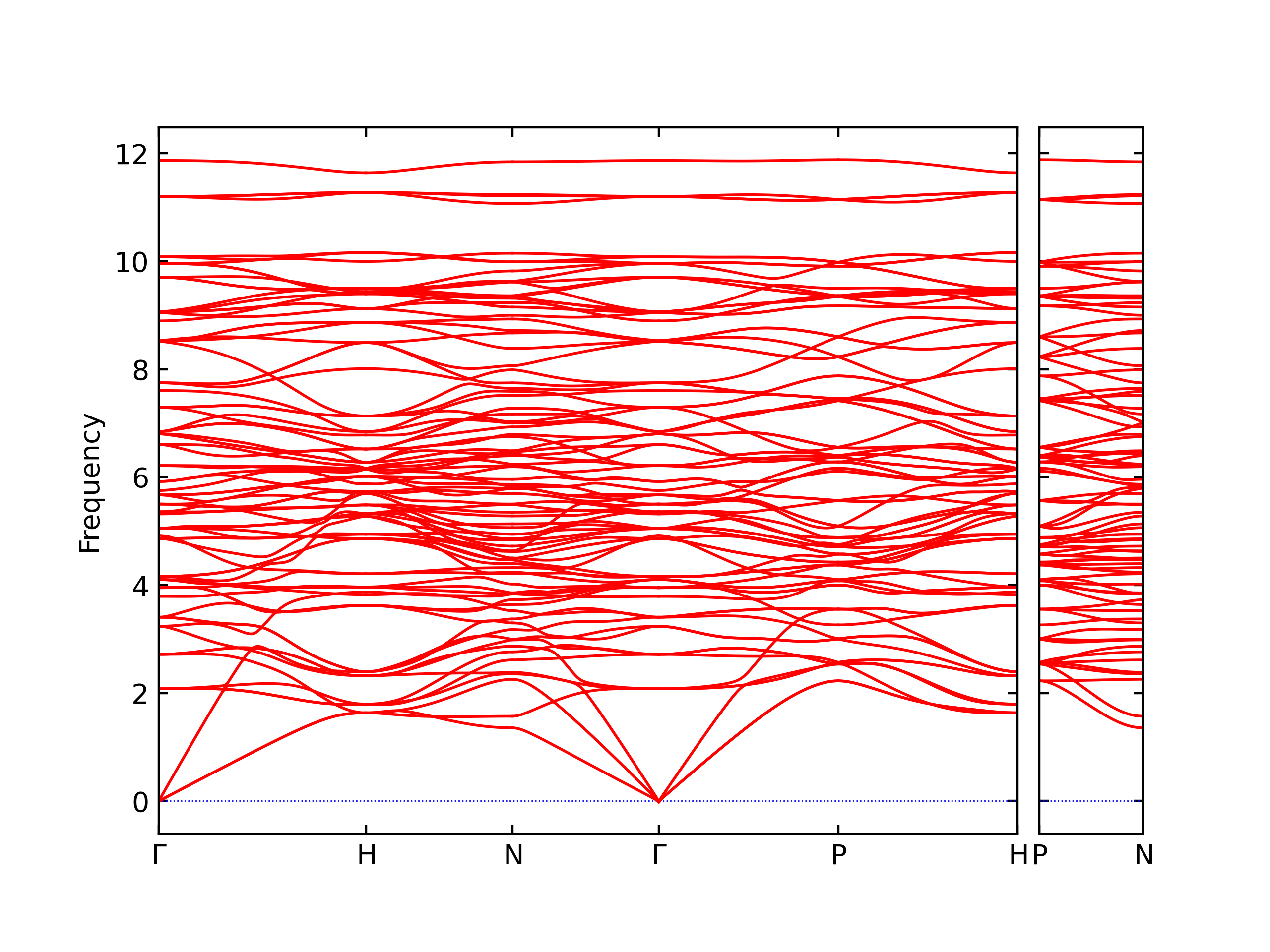
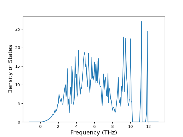
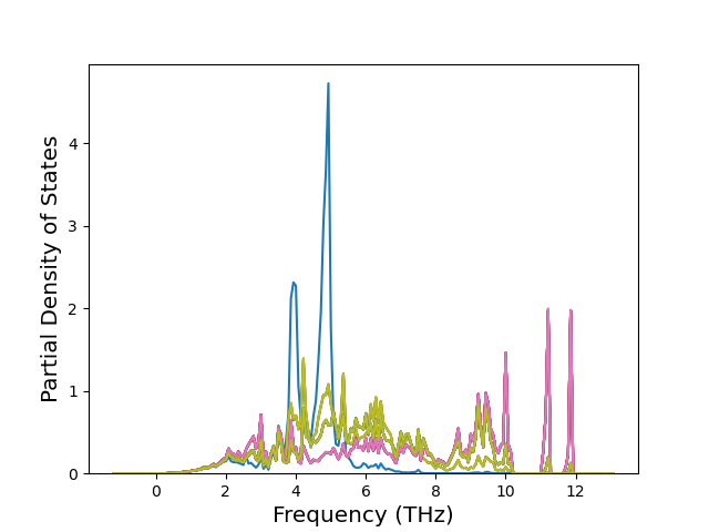
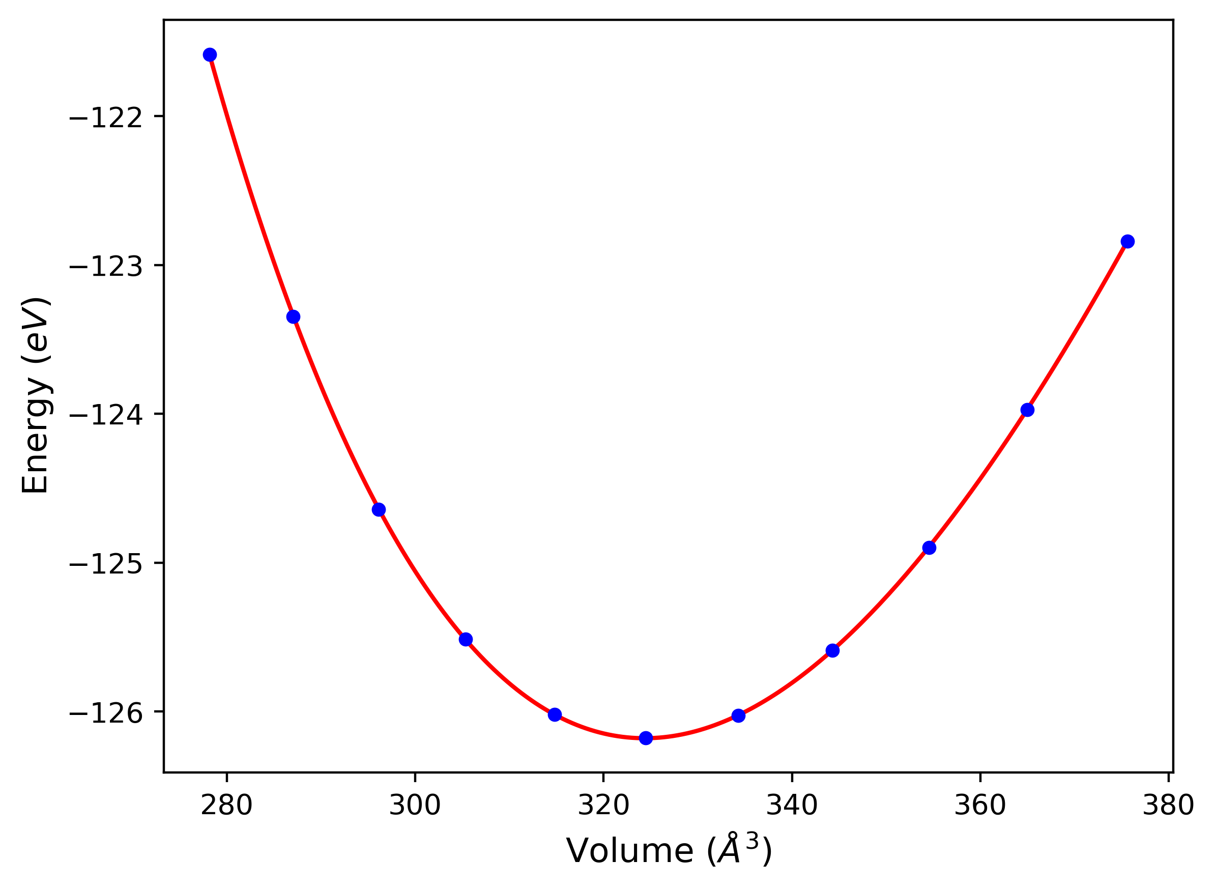
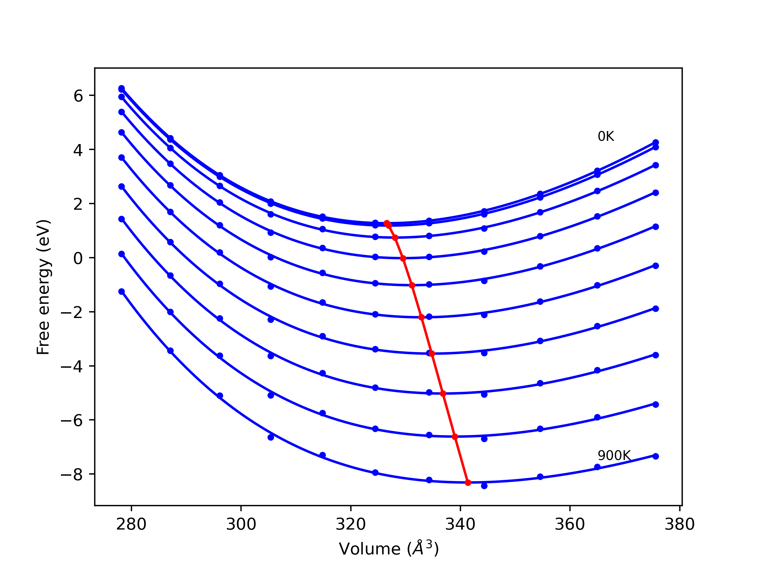
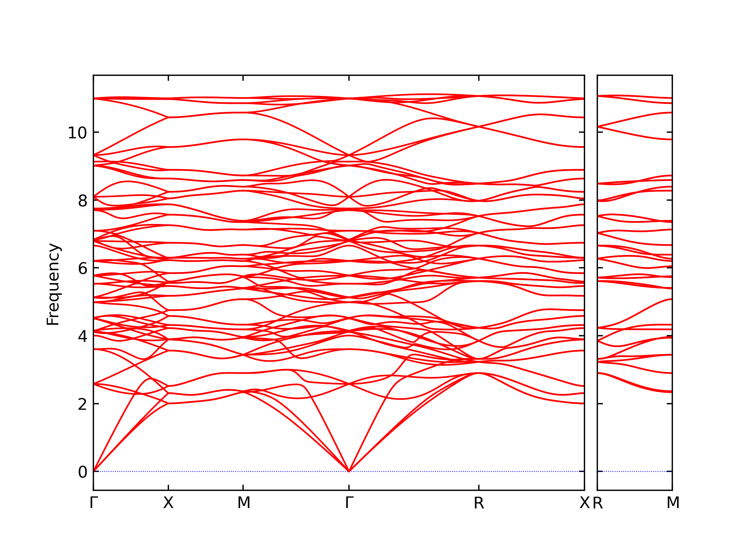
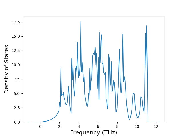
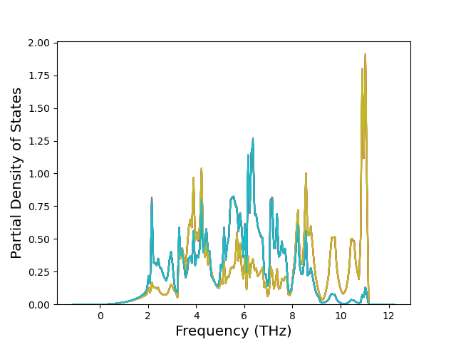
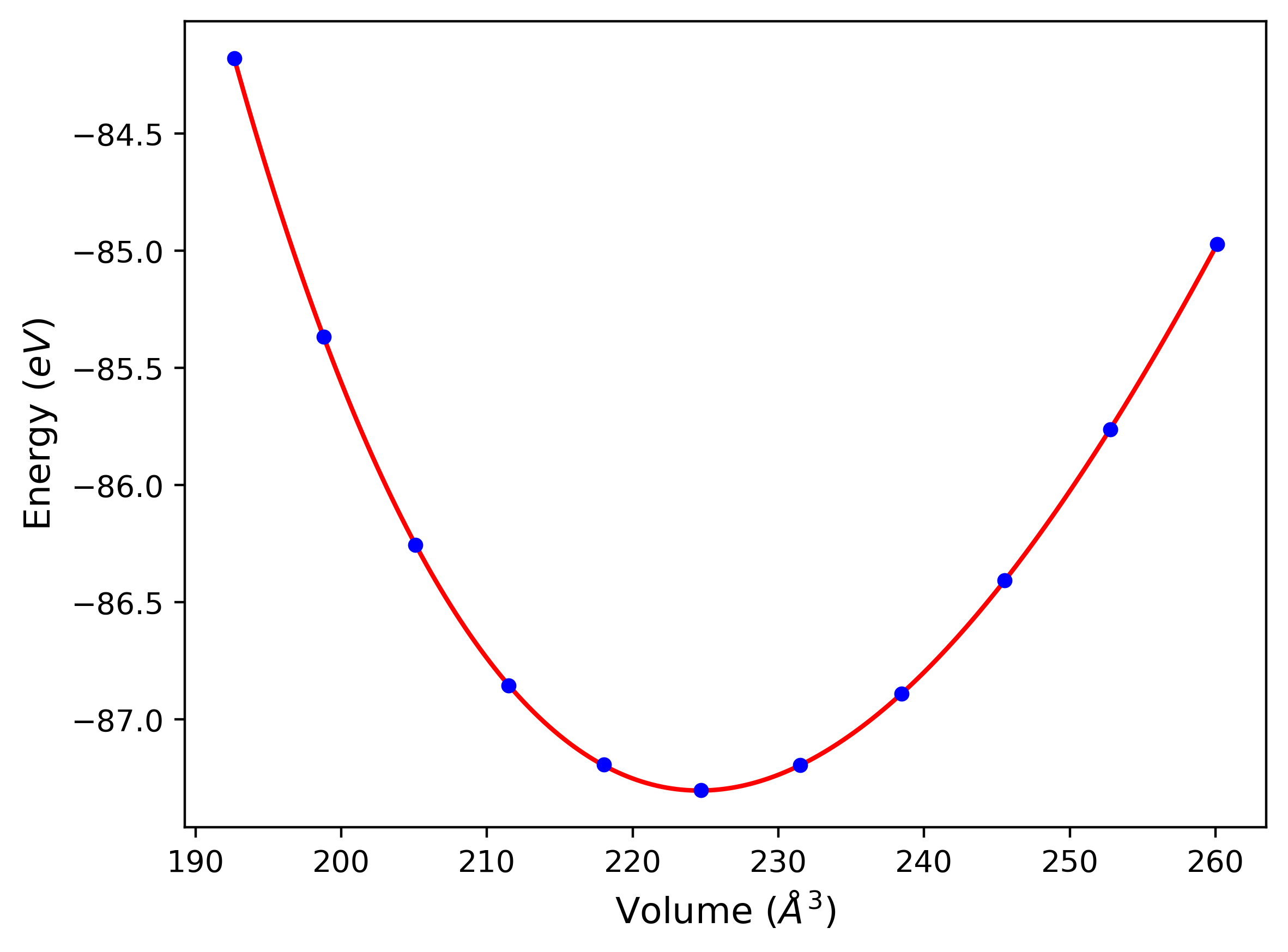
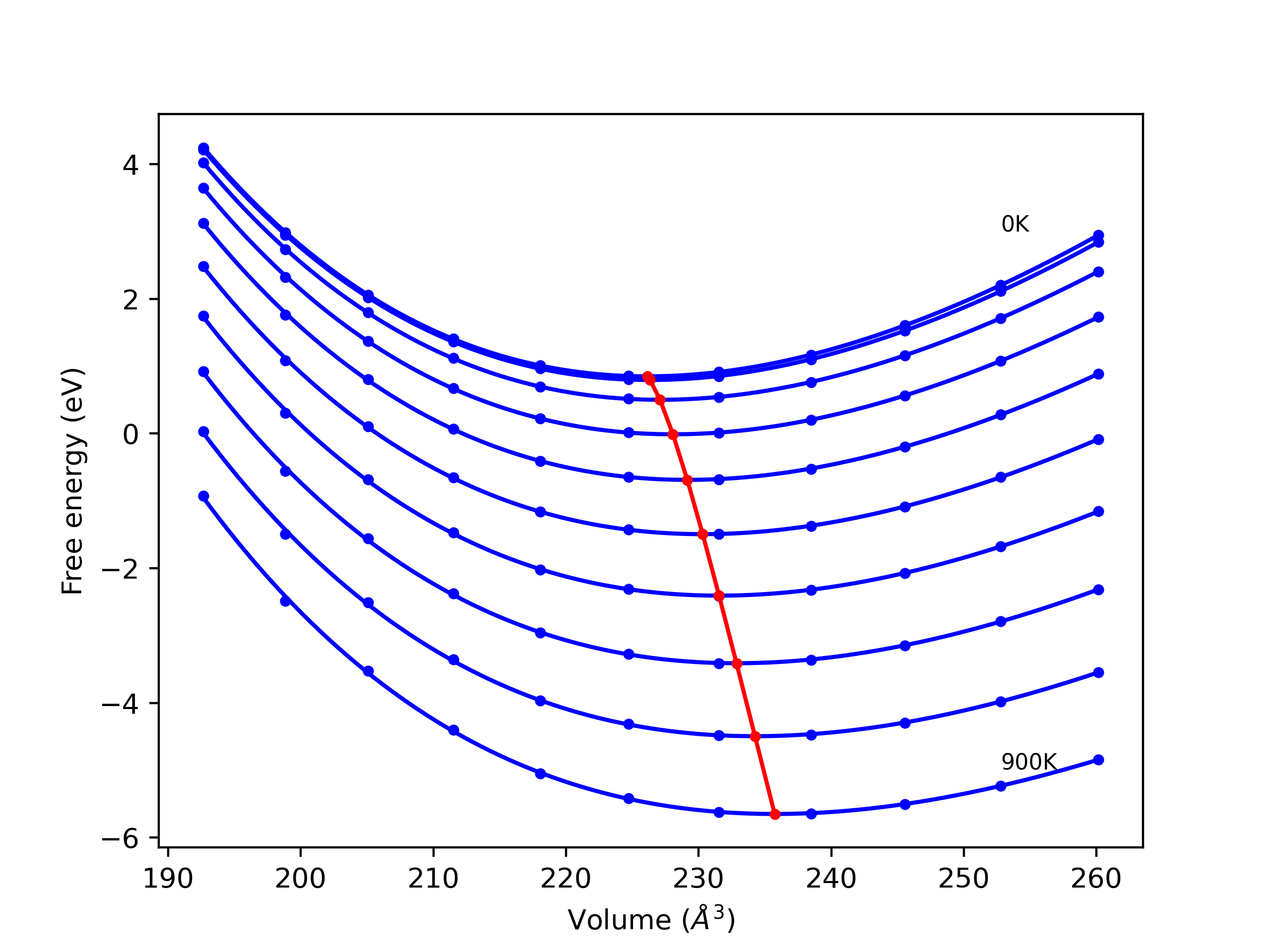
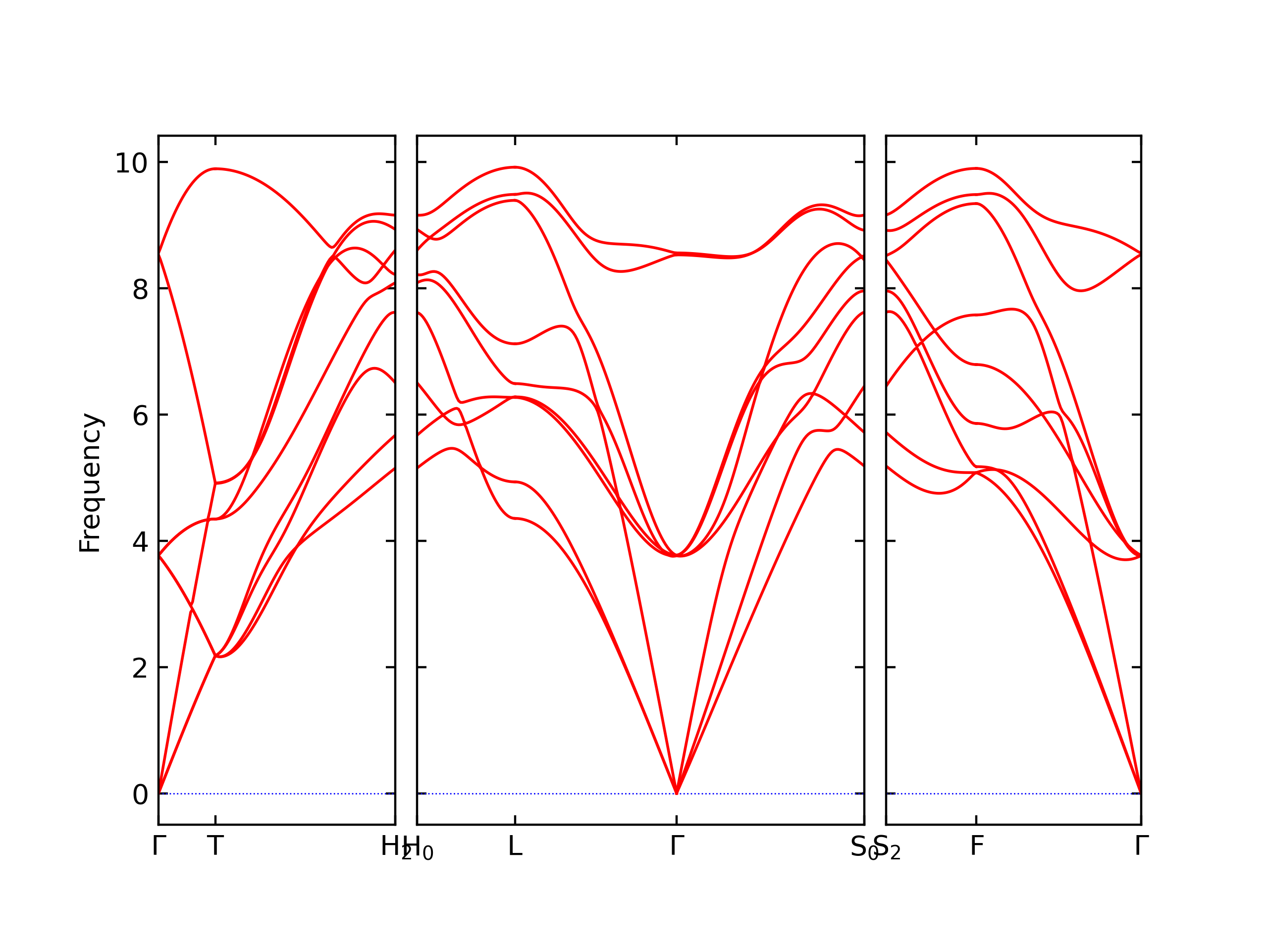
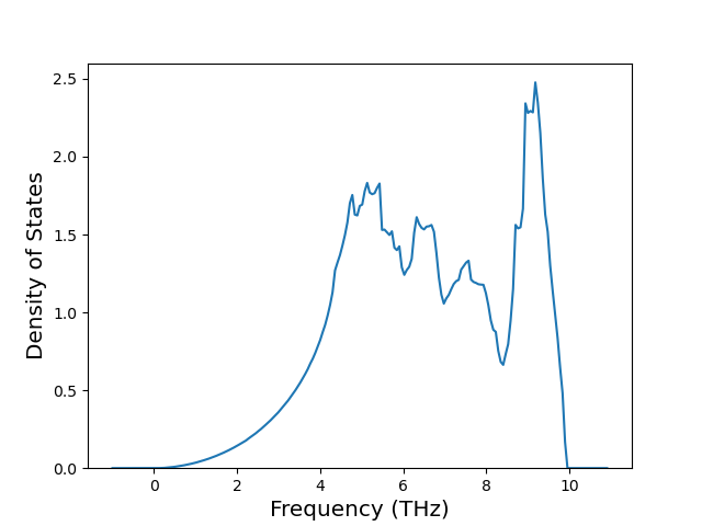
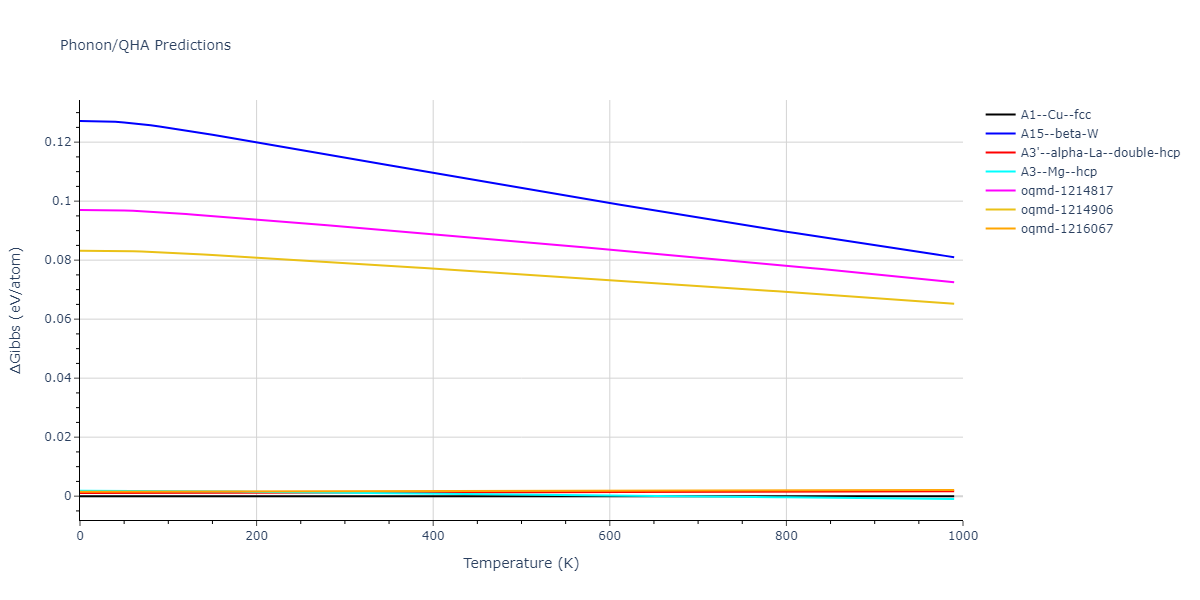
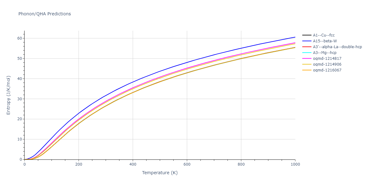
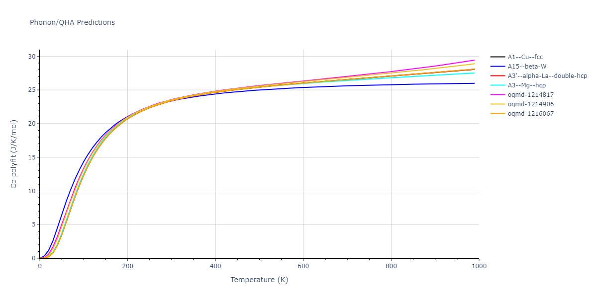
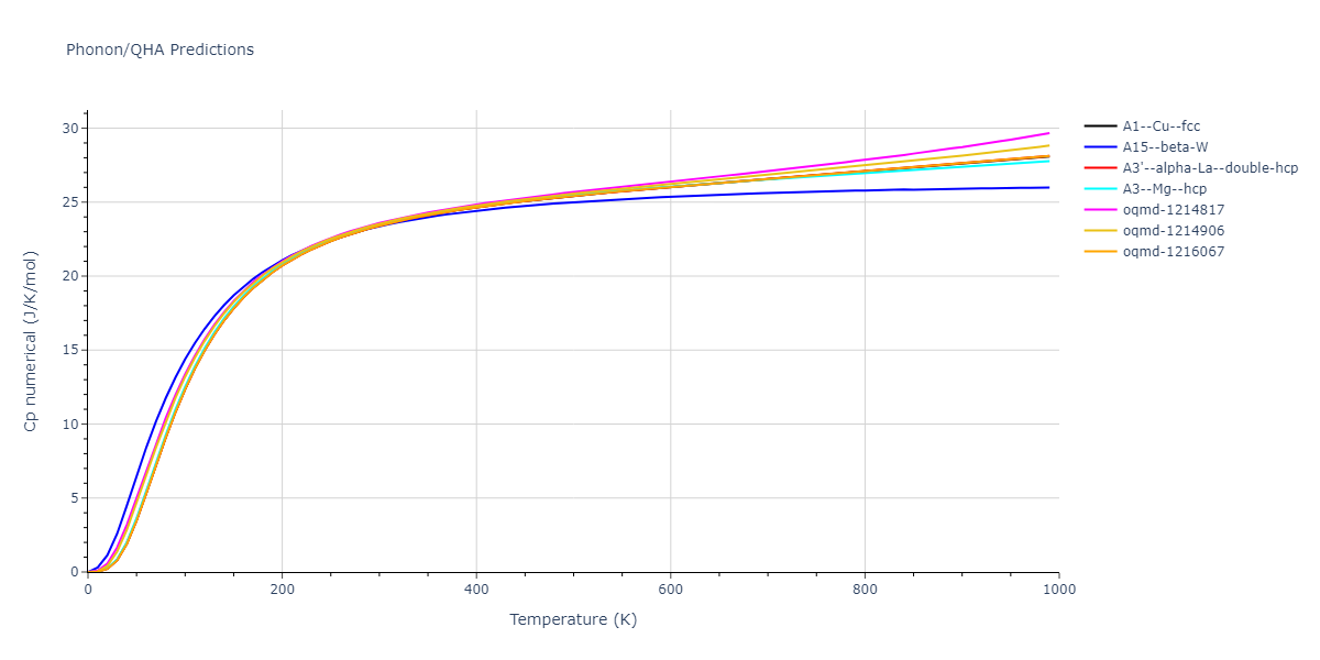
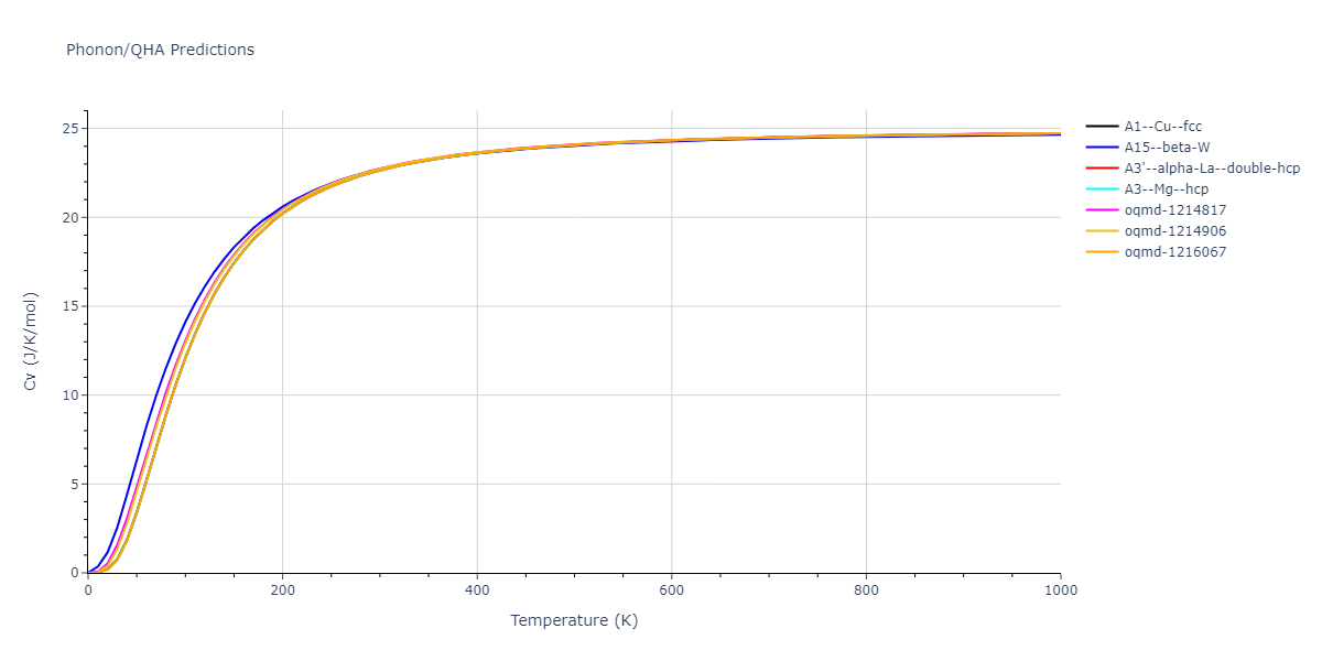
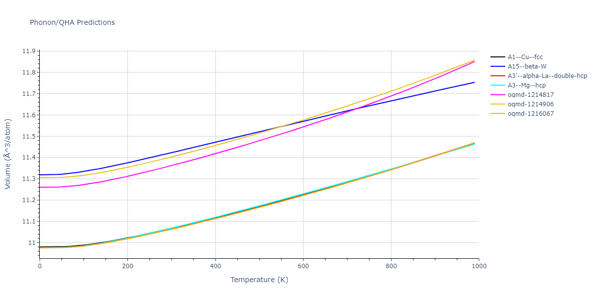
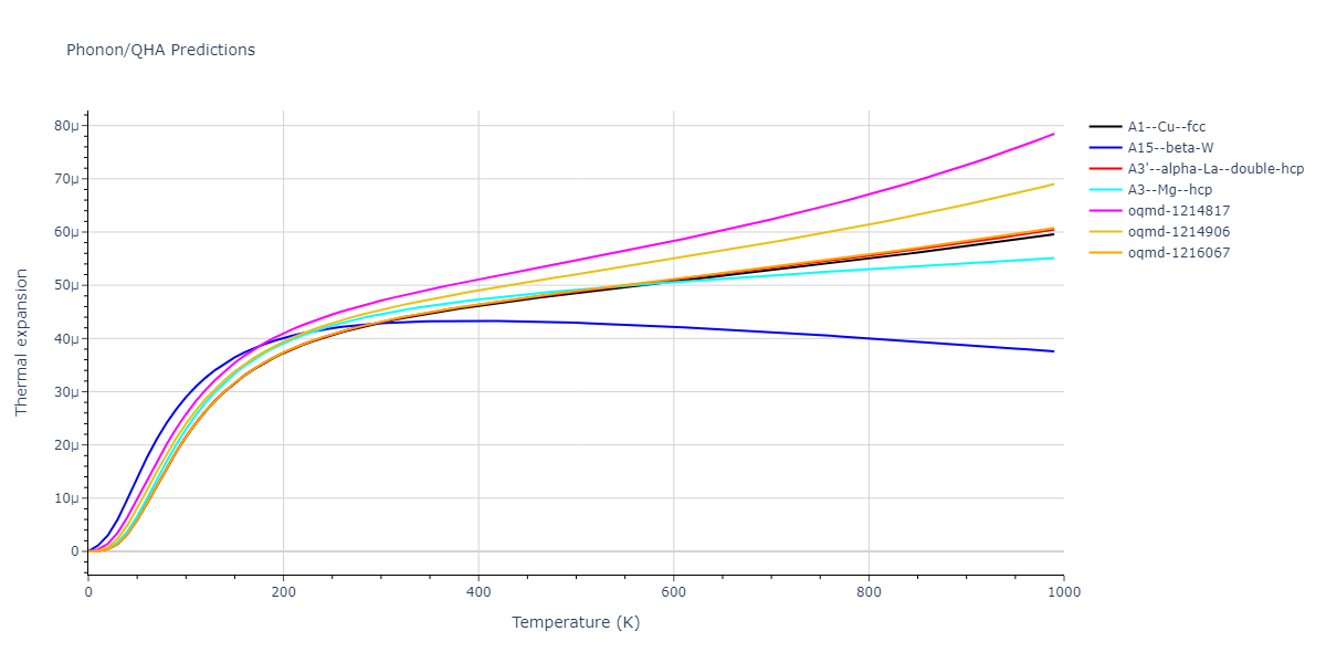
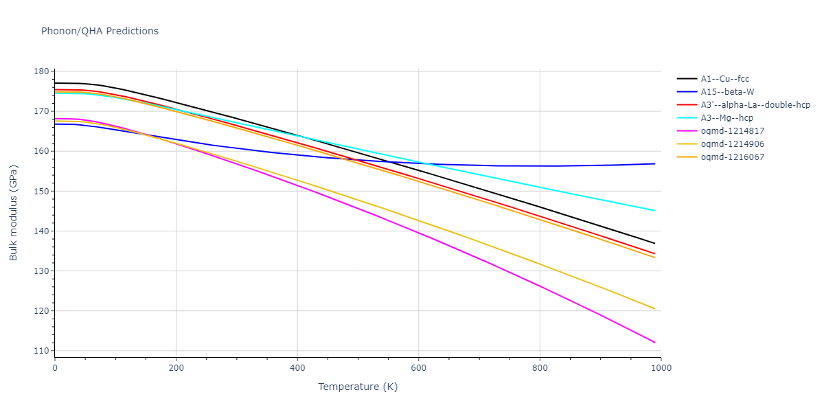
Phonon and Quasi-Harmonic Approximation Predictions
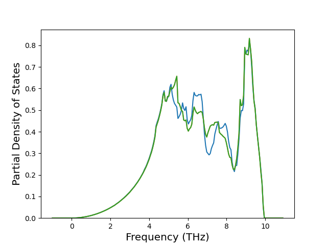
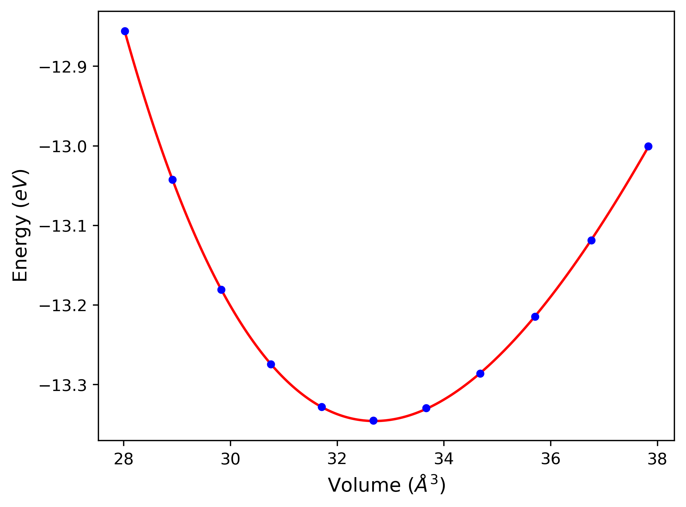
Phonon band structures and crystal properties estimated from quasi-harmonic approximation (QHA) calculations are displayed for select crystals. The calculations were performed using phonopy and LAMMPS. For the phonon calculations, 3x3 supercells of the potential-specific relaxed crystals were used. The QHA calculations were based on 11 strain states ranging from -0.05 to 0.05.
The calculation method used is available as the iprPy phonon calculation method.
Notes and Disclaimers:
- The thermodynamic properties estimated from QHA are based on the assumption that only volumetric changes affect the phonon behaviors as the temperature changes. This tends to give good predictions at lower temperatures but ignores anharmonic effects such as phonon coupling and vacancy formation that can be important at higher temperatures.
- Note that direct molecular dynamics (MD) simulations using the same potentials will disagree with the thermodynamics properties listed here for the lowest temperatures. The MD results are purely classical in nature and therefore lack a zero-point energy, whereas the phonon calculations inherently provide a zero-point energy.
- The structures explored here are taken from the dynamically relaxed structures above. Despite the rigorous relaxation method used, some of these structures prove to be unstable once internal deformations are added. The phonon results may reflect this and give bad band gap predictions for these unstable crystals.
- All QHA calculations performed here use the same set of strains which might not be ideal for all crystals. Be sure to check the bulk modulus and Helmholtz vs. volume plots to verify if the QHA strained states are reasonable for each crystal of interest.
- QHA results may not be available for all crystal structures that have phonon results. Missing QHA results indicates an issue either with the strained states or with the QHA calculation itself.
- NIST disclaimer
Version Information:
- 2023-03-14. Phonon and QHA plots added
Band Structures, Density of States, and QHA Verification Plots


Thermodynamic Predictions
Free Surface Formation Energy Predictions
Static free surface formation energies are displayed for select crystals. The values displayed here are obtained by taking a perfect periodic bulk crystal, slicing along a crystallographic plane, and using force minimization to statically relax the surfaces. The free surface formation energy is computed by comparing the energy of the defect system to the bulk system and dividing by the total surface area created by the cut.
The calculation method used is available as the iprPy surface_energy_static calculation method.
Notes and Disclaimers:
- These values are meant to be guidelines for comparing potentials, not the absolute values for any potential's properties. Values listed here may change if the calculation methods are updated due to improvements/corrections. Variations in the values may occur for variations in calculation methods, simulation software and implementations of the interatomic potentials.
- The calculation only performs straight cuts along crystallographic planes and static relaxations. Lower energy configurations may exist that require atomic restructuring of the surfaces.
- Multiple values may be listed for a given plane followed by a number indicating different unique atomic planar cuts for the same theoretical plane.
- NIST disclaimer
Version Information:
- 2019-11-14. Calculations for the alternate #2 plane slices are now different from the #1 plane slices.
- 2019-08-07. Data added.
| Surface | γfs (mJ/m2) |
|---|---|
| (111) | 1435.93 |
| (100) | 1570.30 |
| (332) | 1577.32 |
| (322) | 1593.07 |
| (221) | 1637.86 |
| (211) | 1666.42 |
| (331) | 1685.30 |
| (311) | 1712.67 |
| (110) | 1718.68 |
| (321) | 1745.83 |
| (310) | 1771.86 |
| (320) | 1792.62 |
| (210) | 1804.97 |
Point Defect Formation Energy Predictions
Static point defect formation energies, Ef, and elastic dipole tensors, pij, are displayed for select crystals. Relaxed defect configurations are obtained by taking a 12x12x12 supercell of a perfect periodic bulk crystal, inserting the point defect, and using force minimization to statically relax the atomic positions while keeping the system dimensions constant. Ef is computed by comparing the energy of the defect system to the same number of atoms in a perfect bulk crystal. pij is estimated as the difference in the system's global pressure with and without the defect multiplied by the system's volume.
Simple structural comparisons of the unrelaxed and relaxed defect configurations are used to help determine if the defect structure has relaxed to a different configuration. Relaxed structures that are identified as no longer consistent with the ideal defect definition are excluded from the table below. The only exception to this is if the lowest energy interstitial configuration does not coincide with a known ideal defect, its energies and pressure tensor are included under the listing "relaxed interstitial". The full list of calculation results including the transformed structures and the structural comparison values is included in the csv file available from the "Download raw data" link.
The calculation method used is available as the iprPy point_defect_static calculation method.
Notes and Disclaimers:
- These values are meant to be guidelines for comparing potentials, not the absolute values for any potential's properties. Values listed here may change if the calculation methods are updated due to improvements/corrections. Variations in the values may occur for changes in calculation methods, simulation software and implementations of the interatomic potentials.
- The computed formation energy and elastic dipole tensor values are sensitive to the size of the system used. The 12x12x12 supercell size was selected as it should provide a decent approximation of the true bulk values.
- The tests for identifying configuration relaxations are not guaranteed to be comprehensive or suitable for all point defect types. The table only shows the point defects that are consistent with the ideal configurations for that defect type, and the lowest energy interstitial.
- The "relaxed interstitial" label indicates that the structure is not consistent with any of the known ideal interstitial configurations. No information is provided as to what that relaxed strucutre is, whether it is an unknown structure, a "near"-ideal defect, or a collapse to amorphous.
- NIST disclaimer
| Point Defect | Ef (eV) | p11 (eV) | p22 (eV) | p33 (eV) | p12 (eV) | p13 (eV) | p23 (eV) |
|---|---|---|---|---|---|---|---|
| vacancy | 1.631 | -1.557 | -1.557 | -1.557 | -0.000 | -0.000 | -0.000 |
| 1nn divacancy | 3.034 | -3.925 | -2.951 | -2.951 | -0.000 | -0.000 | 0.001 |
| 2nn divacancy | 3.233 | -3.345 | -3.345 | -3.460 | -0.000 | -0.000 | -0.000 |
| 100 dumbbell | 4.527 | 26.229 | 26.229 | 25.268 | -0.000 | 0.000 | -0.000 |
| 110 dumbbell | 4.869 | 30.656 | 24.668 | 24.668 | -0.000 | -0.000 | 15.607 |
| 111 dumbbell | 5.173 | 27.132 | 27.132 | 27.132 | 5.234 | 5.234 | 5.234 |
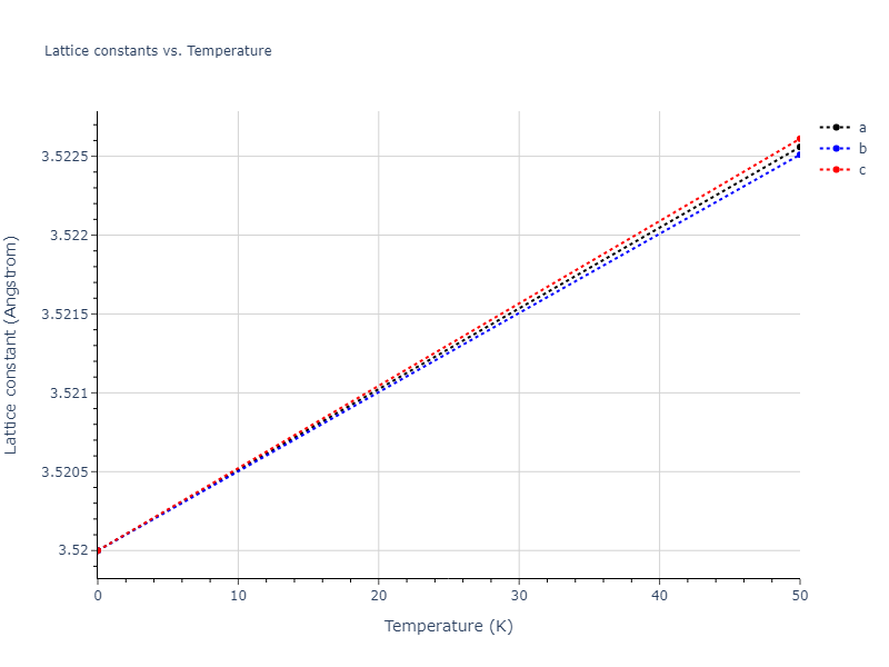
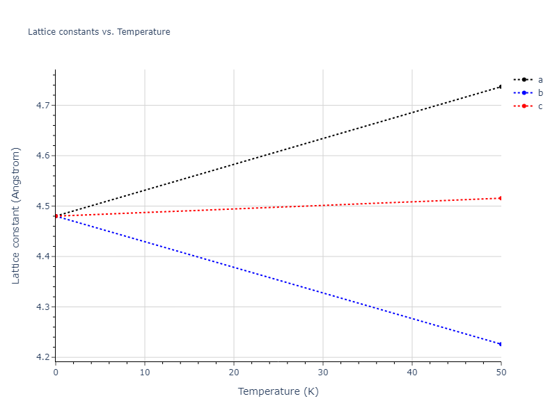
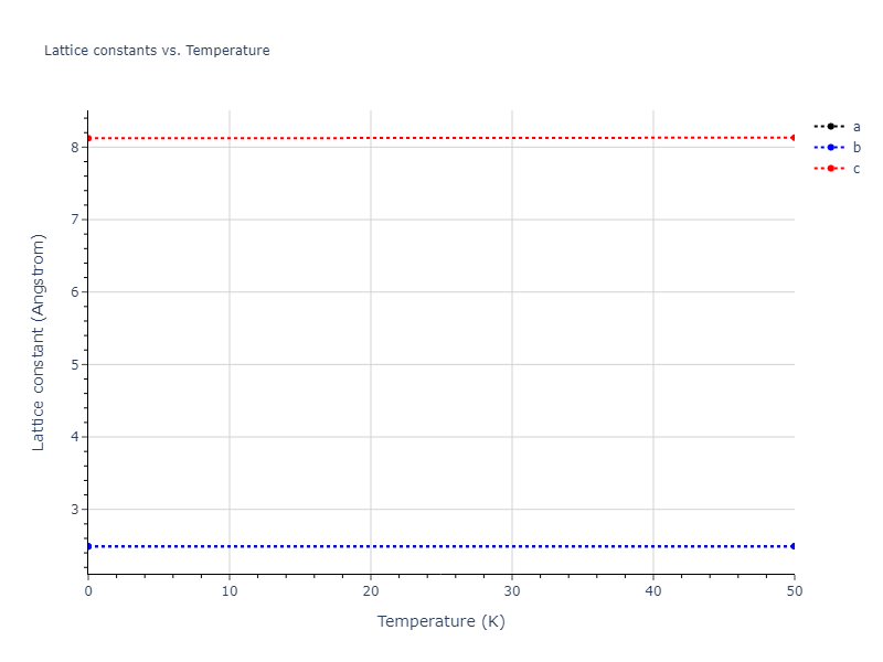
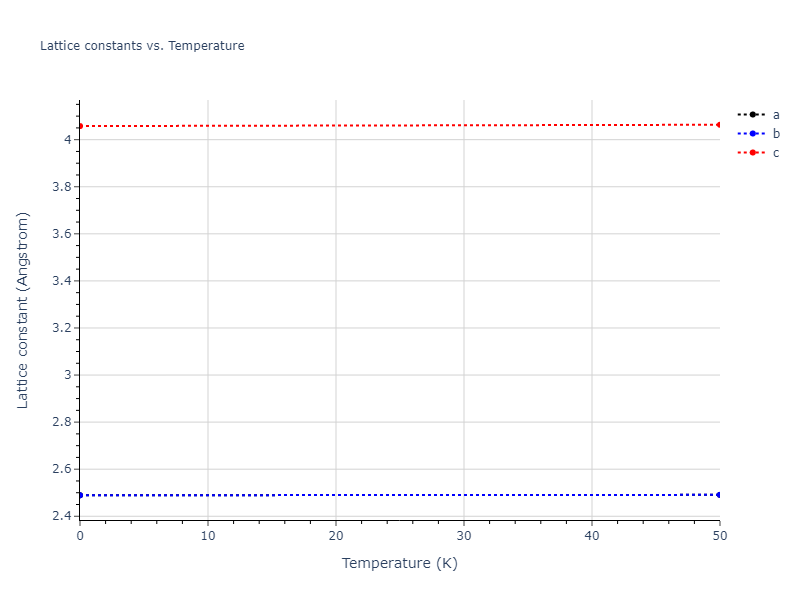
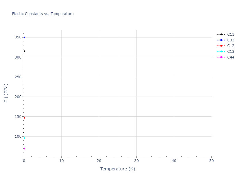
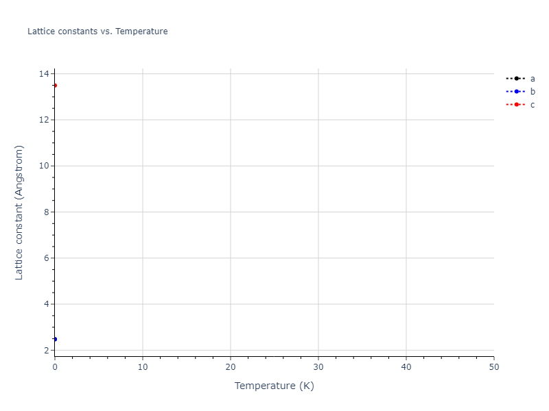
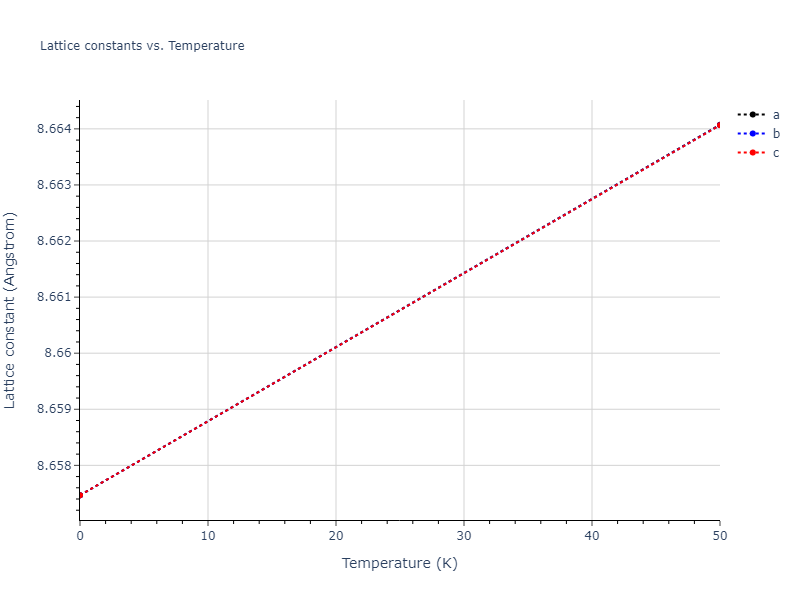
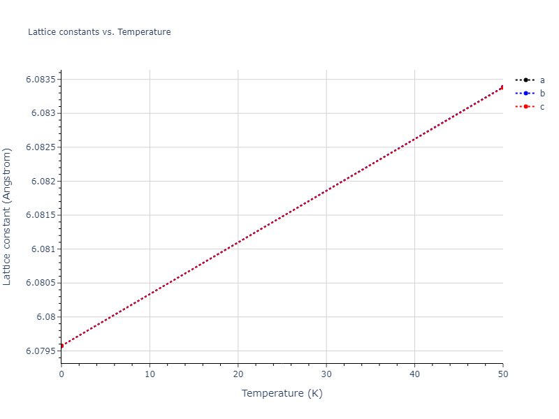
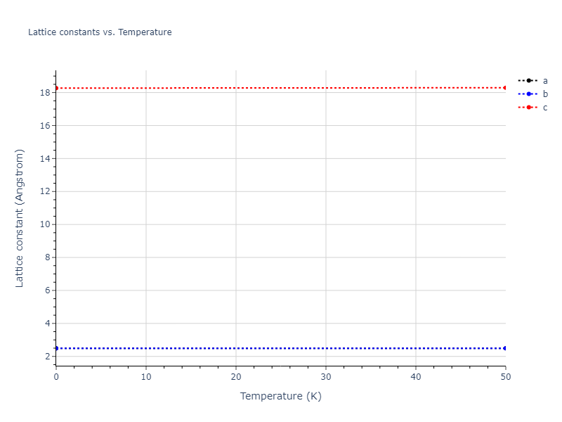
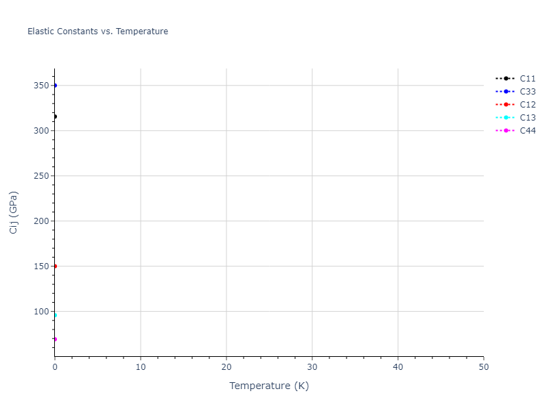
MD Solid Property Predictions
Plots of lattice and elastic constants are shown as a function of temperature. The 0K points were taken from the Crystal Structure Predictions and the Elastic Constants Predictions sections above for the unique crystal structures relaxed with the "dynamic" method. Starting from the 0 K relaxed crystal unit cells, supercell systems are created by replicating all three dimensions by the same multiplier to achieve at least 4000 atoms. The systems are then relaxed at 50 K and zero pressure using 1 million NPT steps. Lattice constants are estimated by averaging the measured box dimensions. Temperatures are iteratively increased by 50 K, with each subsequent relaxation calculation starting from the final atomic configuration at the previous temperature and relaxing for another 1 million steps.
The elastic constants are calculated using the deformation–fluctuation hybrid method. Starting from the final atomic configurations of the dynamic relaxations, the system is allowed to evolve at constant volume with a Langevin thermostat. The Born matrix is computed during this run by evaluating how the atomic forces would vary due to applied linear strain fields. The elastic constants can then be estimated using the averaged Born matrix values and the averaged stresses on the system.
The calculation methods used are available as the iprPy relax_dynamic and elastic_constants_dynamic calculation methods.
Clicking on the image of a plot will open an interactive version of it in a new tab. The underlying data for the plots can be downloaded by clicking on the links above each plot.
Notes and Disclaimers:
- The maximum temperature shown for a crystal either corresponds to the maximum value that has been computed so far, or the maximum value that the structure is believed to have remained untransformed. The unstable/transformation temperature identification is mostly automated and can miss transitions not associated with large discontinuities in property values with changing temperature.
- For succinctness, the elastic constants displayed here are averaged according to the 0 K structure's crystal symmetry family. If the structures deviate from the expected symmetry at higher temperatures, the values may not be valid. Raw results are available for verification if requested.
- NIST disclaimer
Version Information:
- 2025-08-07. Plots added.
Click on plot to load interactive version
Click on plot to load interactive version


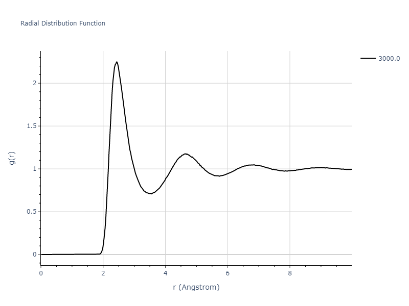
MD Liquid Property Predictions
Plots of radial distribution functions at different temperatures and the temperature-dependent diffusion and viscosity are shown here for elemental liquids. Melt phases are constructed by starting with a 10x10x10 fcc super cell and relaxing with 50,000 NPT steps at zero pressure and a high melting temperature (3000 K for most potentials and elements). Following the melt, liquid structures are relaxed by running NPT for 10,000 steps over which the temperature is dropped by 50 K, then 50,000 NPT at the target temperature to estimate the equilibrium volume, followed by 20,000 NVT steps at the averaged equilibrium volume and target temperature. Structures from the NVT run are sampled to compute the radial distribution function of the liquid at the corresponding temperature.
The final relaxed configurations at each temperature explored are used as the initial configurations for the diffusion and viscosity calculations. For diffusion, the system is integrated for 100 runs of 2,000 NVT steps during which both the mean squared displacement (MSD) and the velocity auto correlation function (VACF) are computed. From these simulations, three estimates of diffusion are computed: one from the MSD of the full 200,000 step run, one in which the MSD is reset for each short run and then averaged, and one from the VACF computed for each short run and averaged. For viscosity, the Green-Kubo method is used which is evaluated during a 1 million step NVT run.
The calculation methods used are available as the iprPy relax_liquid_redo, diffusion_liquid, and viscosity_green_kubo calculation methods.
Clicking on the image of a plot will open an interactive version of it in a new tab. The underlying data for the plots can be downloaded by clicking on the links above each plot.
Notes and Disclaimers:
- The current liquid relaxation has some known issues, and therefore may be recalculated with an improved method later. Most notably, the unconstrained NPT relaxation may lead to one of the periodic dimensions becoming quite small which can negatively affect the simulations and property calculations. Additionally, the relaxations likely need to be longer to reduce the error associated with the measured volume and energy values.
- Values are only displayed down to the last temperature currently calculated, or the last temperature at which the system is believed to remain liquid until the end of all simulations. The transformation temperature is estimated by looking at discontinuities in the measured property values and may incorrectly predict a phase to still be liquid if the discontinuities are small.
- The three diffusion estimates provide a range of prediction values. For MSD, the longer the run the more likely it is that a small number of atoms will diffuse much farther than the rest, which skews the squared displacement higher.
- NIST disclaimer
Version Information:
- 2025-08-07. Plots added. Data should be thought of as preliminary as results may be recalculated later.
Click on plot to load interactive version
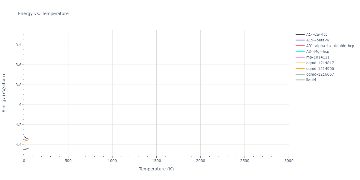
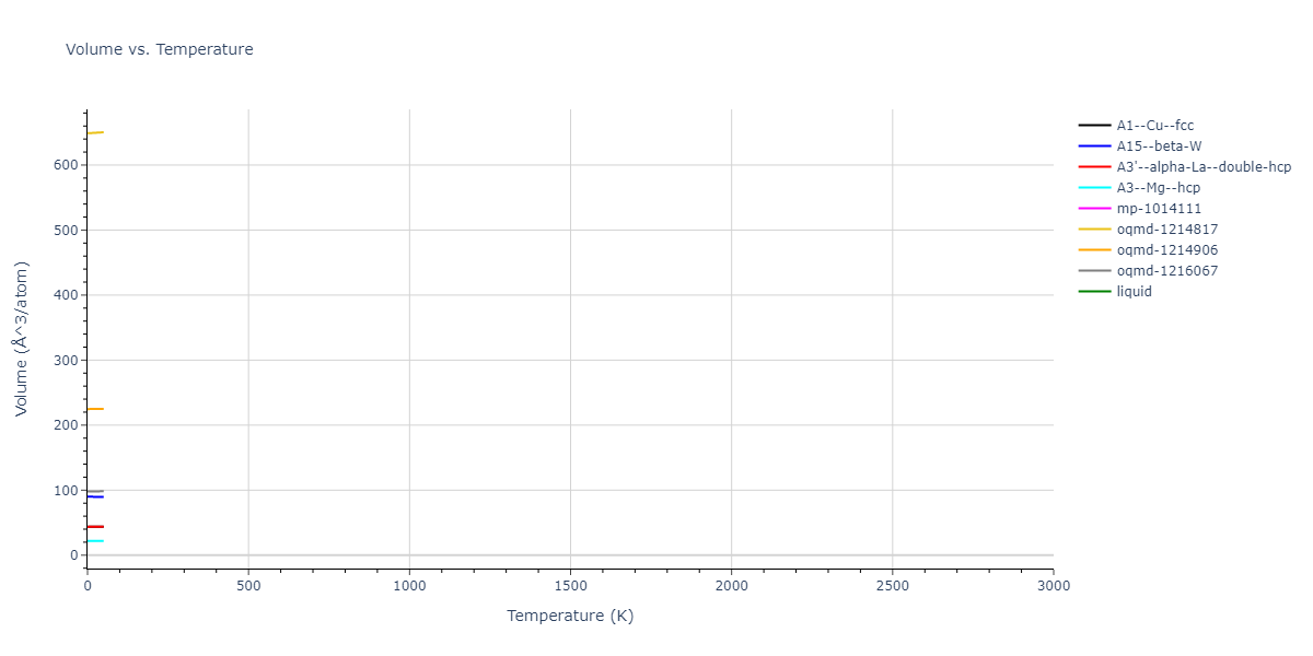
MD Thermodynamic Predictions
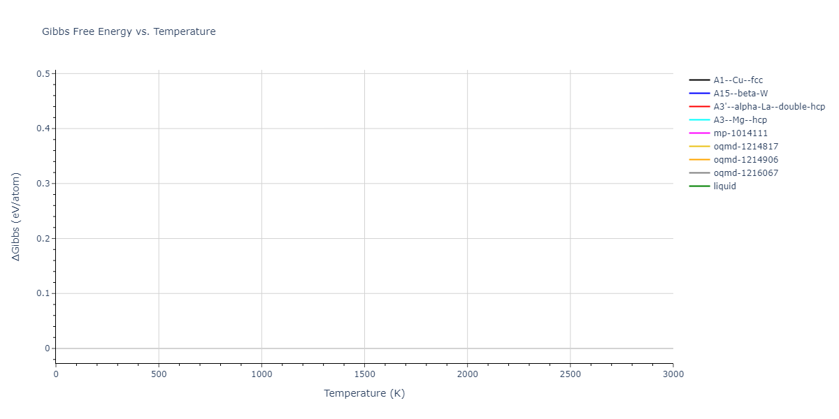
Plots of internal energy, Gibbs free energy, entropy, heat capacity and volume are shown here as a function of temperature for various crystal structures and liquid phases. The included crystal structures correspond to those in the Solid Structures vs. Temperature section, and the liquid phases to those in the Liquid Properties section. Internal energy and volume are taken from the associated structure relaxations mentioned in those previous sections. Constant pressure heat capacity is estimated using 3-point numerical derivatives of enthalpy versus temperature. Note that since all simulations done here are at 0 pressure, internal energy and enthalpy are equivalent.
The Gibbs energies of the phases are estimated using thermodynamic integration between the interatomic potential in question and a simpler model with known Gibbs free energy values. For solids, the reference model is an Einstein solid, while for liquids it is the Uhlenbeck-Ford potential. Besides a short run at the start of the solid calculations to estimate Einstein model spring constants, the two calculations proceed similarly. Starting with the final relaxation configurations, the systems are stabilized for 25,000 steps. Then, over the next 50,000 steps the potential is swapped out for the reference potential. The system is then stabilized for another 25,000 steps with the reference model before a reverse swap of 50,000 steps is performed. The simulation ends with one final 25,000 step stabilization period. From the simulation, the irreversible work of transformation is estimated and used to compute the absolute Gibbs free energy of the target phase and potential relative to the reference potential. Entropy is estimated as the difference in enthalpy and Gibbs free energy and divided by temperature.
The calculation methods used are available as the iprPy relax_dynamic, relax_liquid_redo, free_energy, and free_energy_liquid calculation methods.
Clicking on the image of a plot will open an interactive version of it in a new tab. The underlying data for the plots can be downloaded by clicking on the links above each plot.
Notes and Disclaimers:
- Good free energy estimates require that the initial and final phases before and after the thermodynamic integration remain the same. This is not an issue with the liquid calculations as the Uhlenbeck-Ford model always predicts a liquid, but may be an issue for the solid phase estimates. This is likely to be an issue for non-compact phases which the Einstein model is poor at representing.
- NIST disclaimer
Version Information:
- 2025-08-07. Plots added.