examples.diffusion.electrostatics¶

Solve the Poisson equation in one dimension.

The Poisson equation is a particular example of the steady-state diffusion equation. We examine a few cases in one dimension.

>>> from fipy import CellVariable, Grid1D, Viewer, DiffusionTerm

>>> nx = 200
>>> dx = 0.01
>>> L = nx * dx
>>> mesh = Grid1D(dx = dx, nx = nx)

Given the electrostatic potential $\phi$ ,

>>> potential = CellVariable(mesh=mesh, name='potential', value=0.)

the permittivity $\epsilon$ ,

>>> permittivity = 1

the concentration $C_j$ of the $j^\text{th}$ component with valence $z_j$ (we consider only a single component $C_\text{e}^{-}$ with valence with $z_{\text{e}^{-}} = -1$ )

>>> electrons = CellVariable(mesh=mesh, name='e-')
>>> electrons.valence = -1

and the charge density $\rho$ ,

>>> charge = electrons * electrons.valence
>>> charge.name = "charge"

The dimensionless Poisson equation is

$\nabla\cdot\left(\epsilon\nabla\phi\right) = -\rho = -\sum_{j=1}^n z_j C_j$

>>> potential.equation = (DiffusionTerm(coeff = permittivity)
...                       + charge == 0)

Because this equation admits an infinite number of potential profiles, we must constrain the solution by fixing the potential at one point:

>>> potential.constrain(0., mesh.facesLeft)

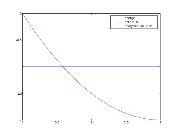
First, we obtain a uniform charge distribution by setting a uniform concentration of electrons $C_{\text{e}^{-}} = 1$ .

>>> electrons.setValue(1.)

and we solve for the electrostatic potential

>>> potential.equation.solve(var=potential)

This problem has the analytical solution

$\psi(x) = \frac{x^2}{2} - 2x$

>>> x = mesh.cellCenters[0]
>>> analytical = CellVariable(mesh=mesh, name="analytical solution",
...                           value=(x**2)/2 - 2*x)

which has been satisfactorily obtained

>>> print(potential.allclose(analytical, rtol = 2e-5, atol = 2e-5))
1

If we are running the example interactively, we view the result

>>> from fipy import input
>>> if __name__ == '__main__':
...     viewer = Viewer(vars=(charge, potential, analytical))
...     viewer.plot()
...     input("Press any key to continue...")

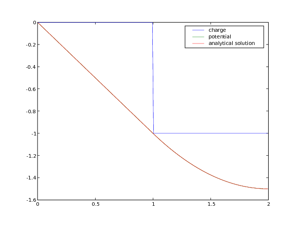
electrostatic potential generated by uniform charge

Next, we segregate all of the electrons to right side of the domain

$C_{\text{e}^{-}} = \begin{cases} 0& \text{for $x \le L/2$,} \\ 1& \text{for $x > L/2$.} \end{cases}$

>>> x = mesh.cellCenters[0]
>>> electrons.setValue(0.)
>>> electrons.setValue(1., where=x > L / 2.)

and again solve for the electrostatic potential

>>> potential.equation.solve(var=potential)

which now has the analytical solution

$\psi(x) = \begin{cases} -x& \text{for $x \le L/2$,} \\ \frac{(x-1)^2}{2} - x& \text{for $x > L/2$.} \end{cases}$

>>> analytical.setValue(-x)
>>> analytical.setValue(((x-1)**2)/2 - x, where=x > L/2)

>>> print(potential.allclose(analytical, rtol = 2e-5, atol = 2e-5))
1

and again view the result

>>> from fipy import input
>>> if __name__ == '__main__':
...     viewer.plot()
...     input("Press any key to continue...")

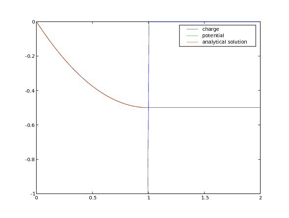
electrostatic potential generated by negative charge on right

Finally, we segregate all of the electrons to the left side of the domain

$C_{\text{e}^{-}} = \begin{cases} 1& \text{for $x \le L/2$,} \\ 0& \text{for $x > L/2$.} \end{cases}$

>>> electrons.setValue(1.)
>>> electrons.setValue(0., where=x > L / 2.)

and again solve for the electrostatic potential

>>> potential.equation.solve(var=potential)

which has the analytical solution

$\psi(x) = \begin{cases} \frac{x^2}{2} - x& \text{for $x \le L/2$,} \\ -\frac{1}{2}& \text{for $x > L/2$.} \end{cases}$

We again verify that the correct equilibrium is attained

>>> analytical.setValue((x**2)/2 - x)
>>> analytical.setValue(-0.5, where=x > L / 2)

>>> print(potential.allclose(analytical, rtol = 2e-5, atol = 2e-5))
1

and once again view the result

>>> if __name__ == '__main__':
...     viewer.plot()

electrostatic potential generated by negative charge on left

Last updated on Jun 27, 2023. Created using Sphinx 6.2.1.