FiPy
FiPyexamples.diffusion.circle
Solve the diffusion equation in a circular domain meshed with triangles.
This example demonstrates how to solve a simple diffusion problem on a non-standard mesh with varying boundary conditions. The Gmsh package is used to create the mesh. Firstly, define some parameters for the creation of the mesh,
>>> cellSize = 0.05
>>> radius = 1.
The cellSize is the preferred edge length of each mesh element and the radius is the radius of the circular mesh domain. In the following code section a file is created with the geometry that describes the mesh. For details of how to write such geometry files for Gmsh, see the gmsh manual.
The mesh created by Gmsh is then imported into FiPy using the
Gmsh2D object.
>>> from fipy import CellVariable, Gmsh2D, TransientTerm, DiffusionTerm, Viewer
>>> from fipy.tools import numerix
>>> mesh = Gmsh2D('''
...               cellSize = %(cellSize)g;
...               radius = %(radius)g;
...               Point(1) = {0, 0, 0, cellSize};
...               Point(2) = {-radius, 0, 0, cellSize};
...               Point(3) = {0, radius, 0, cellSize};
...               Point(4) = {radius, 0, 0, cellSize};
...               Point(5) = {0, -radius, 0, cellSize};
...               Circle(6) = {2, 1, 3};
...               Circle(7) = {3, 1, 4};
...               Circle(8) = {4, 1, 5};
...               Circle(9) = {5, 1, 2};
...               Line Loop(10) = {6, 7, 8, 9};
...               Plane Surface(11) = {10};
...               ''' % locals())
Using this mesh, we can construct a solution variable
>>> phi = CellVariable(name = "solution variable",
...                    mesh = mesh,
...                    value = 0.)
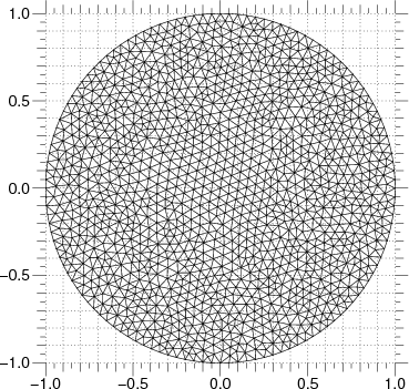
We can now create a Viewer to see the mesh
>>> viewer = None
>>> from fipy import input
>>> if __name__ == '__main__':
...     viewer = Viewer(vars=phi, datamin=-1, datamax=1.)
...     viewer.plotMesh()
We set up a transient diffusion equation
>>> D = 1.
>>> eq = TransientTerm() == DiffusionTerm(coeff=D)
The following line extracts the  coordinate values on the exterior
faces. These are used as the boundary condition fixed values.
coordinate values on the exterior
faces. These are used as the boundary condition fixed values.
>>> X, Y = mesh.faceCenters
>>> phi.constrain(X, mesh.exteriorFaces)
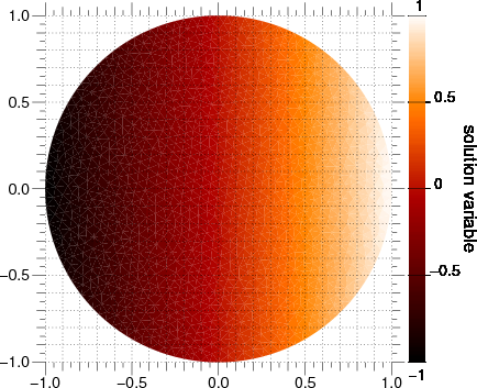
We first step through the transient problem
>>> timeStepDuration = 10 * 0.9 * cellSize**2 / (2 * D)
>>> steps = 10
>>> from builtins import range
>>> for step in range(steps):
...     eq.solve(var=phi,
...              dt=timeStepDuration)
...     if viewer is not None:
...         viewer.plot()
If we wanted to plot or analyze the results of this calculation with another application, we could export tab-separated-values with
TSVViewer(vars=(phi, phi.grad)).plot(filename="myTSV.tsv")
x	y	solution variable	solution variable_grad_x	solution variable_grad_y
0.975559734792414	0.0755414402612554	0.964844363287199	-0.229687917881182	0.00757854476106331
0.0442864953037566	0.79191893162384	0.0375859836421991	-0.773936613923853	-0.205560697612547
0.0246775505084069	0.771959648896982	0.020853932412869	-0.723540342405813	-0.182589694334729
0.223345558247991	-0.807931073108895	0.203035857140125	-0.777466238738658	0.0401235242511506
-0.00726763301939488	-0.775978916110686	-0.00412895434496877	-0.650055516507232	-0.183112882869288
-0.0220279064527904	-0.187563765977912	-0.012771874945585	-0.35707168379437	-0.056072788439713
0.111223320911545	-0.679586798311355	0.0911595298310758	-0.613455176718145	0.0256182541329463
-0.78996770899909	-0.0173672729866294	-0.693887874335319	-1.00671109050419	-0.127611490372511
-0.703545986179876	-0.435813500559859	-0.635004192597412	-0.896203033957194	-0.00855563518923689
0.888641841567831	-0.408558914368324	0.877939107374768	-0.32195762184087	-0.22696791637322
0.38212257821916	-0.51732949653553	0.292889724306196	-0.854466141879776	0.199715815696975
-0.359068256998365	0.757882581524374	-0.323541041763627	-0.870534227755687	0.0792631912863636
-0.459673905457569	-0.701526587772079	-0.417577664032421	-0.725460726303266	-0.119132299176163
-0.338256179134518	-0.523565732643067	-0.254030052182524	-0.923505840608445	-0.192224240688976
0.87498754712638	0.174119064688993	0.836057900916614	-1.11590500805745	-0.211010116496191
-0.484106960369249	0.0705987421869745	-0.319827850867342	-0.867894407968447	0.051246727010685
-0.0221203060940465	-0.216026820080053	-0.0152729438559779	-0.341246696530392	-0.0538476142281317
The values are listed at the cell centers. Particularly for irregular meshes, no specific ordering should be relied upon. Vector quantities are listed in multiple columns, one for each mesh dimension.
This problem again has an analytical solution that depends on the error function, but it’s a bit more complicated due to the varying boundary conditions and the different horizontal diffusion length at different vertical positions
>>> x, y = mesh.cellCenters
>>> t = timeStepDuration * steps
>>> phiAnalytical = CellVariable(name="analytical value",
...                              mesh=mesh)
>>> x0 = radius * numerix.cos(numerix.arcsin(y))
>>> try:
...     from scipy.special import erf
...     ## This function can sometimes throw nans on OS X
...     ## see http://projects.scipy.org/scipy/scipy/ticket/325
...     phiAnalytical.setValue(x0 * (erf((x0+x) / (2 * numerix.sqrt(D * t)))
...                                  - erf((x0-x) / (2 * numerix.sqrt(D * t)))))
... except ImportError:
...     print("The SciPy library is not available to test the solution to \
... the transient diffusion equation")
>>> print(phi.allclose(phiAnalytical, atol = 7e-2))
1
>>> from fipy import input
>>> if __name__ == '__main__':
...     input("Transient diffusion. Press <return> to proceed...")
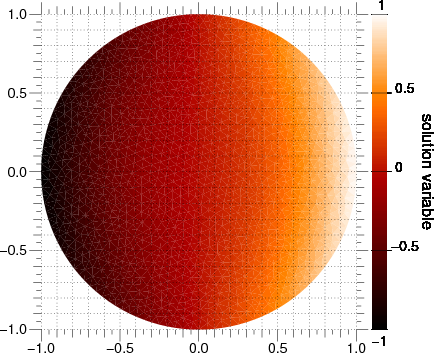
As in the earlier examples, we can also directly solve the steady-state diffusion problem.
>>> DiffusionTerm(coeff=D).solve(var=phi)
The values at the elements should be equal to their x coordinate
>>> print(phi.allclose(x, atol = 0.03))
1
Display the results if run as a script.
>>> from fipy import input
>>> if viewer is not None:
...     viewer.plot()
...     input("Steady-state diffusion. Press <return> to proceed...")