examples.diffusion.nthOrder.input4thOrder1D¶

Solve a fourth-order diffusion problem.

This example uses the DiffusionTerm class to solve the equation

$\frac{\partial^4 \phi}{\partial x^4} = 0$

on a 1D mesh of length

>>> L = 1000.

We create an appropriate mesh

>>> from fipy import CellVariable, Grid1D, NthOrderBoundaryCondition, DiffusionTerm, Viewer, GeneralSolver

>>> nx = 500
>>> dx = L / nx
>>> mesh = Grid1D(dx=dx, nx=nx)

and initialize the solution variable to 0

>>> var = CellVariable(mesh=mesh, name='solution variable')

For this problem, we impose the boundary conditions:

$\phi &= \alpha_1 \quad \text{at $x = 0$} \\ \frac{\partial \phi}{\partial x} &= \alpha_2 \quad \text{at $x = L$} \\ \frac{\partial^2 \phi}{\partial x^2} &= \alpha_3 \quad \text{at $x = 0$} \\ \frac{\partial^3 \phi}{\partial x^3} &= \alpha_4 \quad \text{at $x = L$.}$

or

>>> alpha1 = 2.
>>> alpha2 = 1.
>>> alpha3 = 4.
>>> alpha4 = -3.

>>> BCs = (NthOrderBoundaryCondition(faces=mesh.facesLeft, value=alpha3, order=2),
...        NthOrderBoundaryCondition(faces=mesh.facesRight, value=alpha4, order=3))
>>> var.faceGrad.constrain([alpha2], mesh.facesRight)
>>> var.constrain(alpha1, mesh.facesLeft)

We initialize the steady-state equation

>>> eq = DiffusionTerm(coeff=(1, 1)) == 0

>>> import fipy.solvers.solver
>>> if fipy.solvers.solver  == 'petsc':
...     solver = GeneralSolver(precon='lu')
... else:
...     solver = GeneralSolver()

We perform one implicit timestep to achieve steady state

>>> eq.solve(var=var,
...          boundaryConditions=BCs,
...          solver=solver)

The analytical solution is:

$\phi = \frac{ \alpha_4 }{6} x^3 + \frac{ \alpha_3 }{2} x^2 + \left( \alpha_2 - \frac{ \alpha_4 }{2} L^2 - \alpha_3 L \right) x + \alpha_1$

or

>>> analytical = CellVariable(mesh=mesh, name='analytical value')
>>> x = mesh.cellCenters[0]
>>> analytical.setValue(alpha4 / 6. * x**3 + alpha3 / 2. * x**2 + \
...                     (alpha2 - alpha4 / 2. * L**2 - alpha3 * L) * x + alpha1)

>>> print(var.allclose(analytical, rtol=1e-4))
1

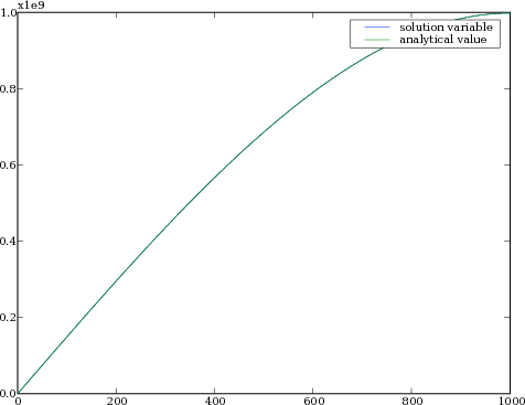
If the problem is run interactively, we can view the result:

>>> if __name__ == '__main__':
...     viewer = Viewer(vars=(var, analytical))
...     viewer.plot()

Last updated on Jun 27, 2023. Created using Sphinx 6.2.1.