OOF: Finite Element Analysis of Microstructures

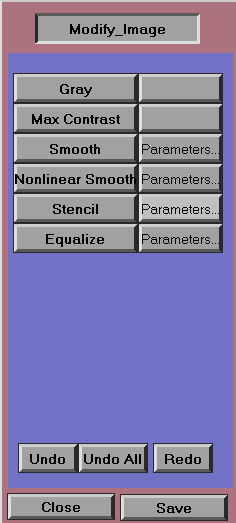
Modify Image Dashboard

Table of Contents	Modify Image Dashboard	OOF home
Prev	The Dashboards	Next

Modify Image Dashboard

Modify Image Dashboard -- Image manipulation tools

Synopsis

There are many commercial and public domain software tools for modifying an image. We constantly found ourselves modifying images outside of ppm2oof and then importing them to make the mashing and material selection more efficient. For this reason, we decided to incorporate a small subset of the functionality of the many image modification tools into ppm2oof.

Figure 3.7. The Modify Image Dashboard

One advantage of including an image modification suite with ppm2oof is that images can be stacked with the Image Gallery dashboard. The groups of pixels that are selected by a Burn or Demography command are referenced by their position only, so selecting a pixel in one image also selects the pixel at the same position in all other images. Therefore, for example, it may be useful to use an edge detection image modification, load the resulting image into the image gallery and then make pixel groups or materials identification based on that image, and use a maximum contrast image manipulation method for other pixel groupings.

Clicking on the large buttons on the left edge of the dashboard performs the image modifications. The smaller buttons next to them bring up Function Windows that allow you to set the parameters used by the modifcation operations. To set parameters, you need to enter their values in the Function Window and press the large button at the top of the window. Setting parameters does not perform the modification--you still have to click on the lefthand button in the dashboard to actually do anything useful.

The image modification tools are illustrated here by applying them to the test image shown in Figure 3.8. . Note that the image is noisy and has a smooth featureless background gradient beneath some sharp features (the letters "OOF" in the lower right corner) and some slightly blurry features (the antialiased letters "OOF" in the upper left corner). The images are displayed here larger than life, to make it easier to see the effects.

Figure 3.8.

The test image used to demonstrate the image modification tools.

Figure 3.9.

The test image Figure 3.8. after 5 iterations of the smooth algorithm with dt=0.1. The sharp edges have been blurred.

Figure 3.10.

The test image Figure 3.8. after 15 iterations of the nonlinear smoothing algorithm with dt=0.1 and alpha=1. The noise reduction is comparable to that achieved with the linear smoothing algorithm, but the sharp borders have been preserved.

Figure 3.11.

The result of applying the laplacian stencil to the test image Figure 3.8. . The smooth gradient has been eliminated (among other features...)

Figure 3.12.

The result of applying the blur stencil to the test image Figure 3.8. .

Figure 3.13.

The result of applying the smooth stencil to the test image Figure 3.8. .

Figure 3.14.

The result of applying the sharpen stencil to the test image Figure 3.8. . Note that the edges of the antialiased letters in the upper left are more distinct, and the edges of the sharp letters in the lower right have acquired a halo. The background noise has increased as well.

Figure 3.15.

The result of applying the edge_find stencil to the test image Figure 3.8. . The distinct edges have become white.

Figure 3.16.

The result of applying the edge_enhance_1 stencil to the test image Figure 3.8. . Edges (and noise) have become sharper, but the background gradient hasn't been lost as it has in Figure 3.15. .

Figure 3.17.

The result of applying the edge_enhance_2 stencil to the test image Figure 3.8. . Noise has been enhanced less than in Figure 3.16.

Figure 3.18.

The result of applying the equalize tool to the test image Figure 3.8. . The window widths were set to 10. The upper left corner is too dark and the lower right corner is too light as a result of the way the algorithm handles the edges of the image.

Dashboard Components

Gray

Convert current image to gray scale. The map is from

(R[0,255], G[0,255], B[0,255]) ⅓(R + G + B).

Max Contrast

Ensure that entire range of brightness is represented in the image. All RGB components of all colors are scaled and shifted so that the minimum component is 0 and the maximum is 255. All color components of all pixels are scaled and shifted by the same amount.

Smooth

Smooth (blur) the image by treating each color component c as a diffusing field on a square lattice, and solve the diffusion equation,

∂ c/∂ t = ∇² c

by Euler's method. The result for test image Figure 3.8. is shown in Figure 3.9.

The parameters are:

dt: The timestep to use when solving the diffusion equation. Note that Euler's method on the diffusion equation is unstable for large timesteps. If your interest is in long-time solutions of the diffusion equation, you should be using something other than ppm2oof! Default: 0.1
nsteps: How many time steps to take. Default: 5

Nonlinear Smooth

The diffusion equation used by Smooth will, if iterated repeatedly, completely obliterate all features of the image. At the suggestion of Allen Tannenbaum of the University of Minnesota, we have implemented a non-linear smoothing algorithm, in which the color components diffuse faster perpendicular to color gradients:

∂ c/∂ t = [( c_xx c_y² - 2 c_x c_y c_xy + c_x² c_yy)/ (1 + (c_x² + c_y²)) ]^{⅓}.

This tends to preserve the sharp boundaries between features in an image while reducing the noise within the features. As with Smooth}, the equation is solved by Euler's method, treating each color component c as an independent field. A sample result is shown in Figure 3.10. . Note how the boundaries are still sharp, but have

The Parameters... button allows you to set the following parameters:

dt: The time step used in Euler's method. The method is unstable if dt is too big. Default: 0.1
alpha: The parameter appearing in eq.~\ref{eq:nonlindiff}. Default: 1
nsteps: How many timesteps to take. Default: 5

Stencil

Replace each RGB component of each pixel by computing the value of a stencil applied to the pixel and its neighbors. A stencil (as used here) is a 3x3 array of numerical weights, or mask. The central weight multiplies the pixel's color component, and the eight weights surrounding it multiply the pixel's neighbors in the corresponding directions. The products are totaled, and the pixel is replaced by the result. In other words, if c__ij is a color component (red, green, or blue) of the pixel at (i,j), then

c_i,j Σ_m=-1,0,1 Σ_n=-1,0,1 w_mnc_i+m,j+n.

Different forms for the weight array w_mn lead to different behaviors. Some of the stencils are very similar to each other. Some of them will work better than others on some images. Experimenting with them is a good way to see just what they do.

The Parameters... button lets you set the stencil weights and the number of iterations:

mask

Defines the weight matrix. The choices are:

laplacian

Replaces each color component with the local value of the discrete laplacian of that component. Changes linear gradients in color to black, for example, as shown in Figure 3.11. .

Table 3.1. laplacian weights

0	1	0
1	-4	1
0	1	0

blur

Replaces every pixel with the average of its neighbors. Because the central pixel is not included, the effect is something like looking at the image with your eyes crossed.

Table 3.2. blur weights

1/8	1/8	1/8
1/8	0	1/8
1/8	1/8	1/8

smooth

Just like blur, but less so. The neighbors don't get 100% of the vote. See Figure 3.13.

Table 3.3. smooth weights

1/13	1/13	1/13
1/13	5/13	1/13
1/13	1/13	1/13

sharpen

Increases contrast at edges. Unstable if repeated too much. See Figure 3.14.

Table 3.4. sharpen weights

-1/8	-1/8	-1/8
-1/8	2	-1/8
-1/8	-1/8	-1/8

edge_find

Increases contrast at edges, while making uniformly colored regions dark. See Figure 3.15.

Table 3.5. edge_find weights

-1	-1	-1
-1	8	-1
-1	-1	-1

edge_enhance_1

This works more or less like sharpen. See Figure 3.16.

Table 3.6. edge_enhance_1 weights

-1	-1	-1
-1	9	-1
-1	-1	-1

edge_enhance_2

A slight variation on edge_enhance_1. See Figure 3.17.

Table 3.7. edge_enhance_2 weights

-1/2	-1/2	-1/2
-1/2	5	-1/2
-1/2	-1/2	-1/2

iterations

How many times should the operation be performed? Default: 1

Equalize

This operation attempts to equalize the illumination of an image by making the average brightness in each small window the same as the average brightness B of the whole image. An example is shown in Figure 3.18. . To be precise, for each pixel (i,j), the algorithm computes the local average brightness b_ij} of a window centered on the pixel, and then scales the pixel's color components by the ratio B/b_ij. The window contains all pixels (x,y) such that i-xrange ≤ x ≤ i+xrange and j-yrange ≤ y ≤ j+yrange.

The parameters are:

xrange: The halfwidth of the local averaging window. Default: 10
yrange: The halfheight of the local averaging window. Default: 10

Undo

Reverts to the previous image in the image stack.

Undo All

Reverts to the first image in the image stack.

Redo

Shifts to the next image in the image stack (if it exists).

Mesh Dashboard

The Dashboards

Image Gallery Dashboard