-
Citation: H. Sharifi, and C.D. Wick (2025), "Developing interatomic potentials for complex concentrated alloys of Cu, Ti, Ni, Cr, Co, Al, Fe, and Mn", Computational Materials Science 248, 113595. DOI: 10.1016/j.commatsci.2024.113595.Abstract: Complex concentrated alloys (CCAs) are a new generation of metallic alloys composed of three or more principal elements with physical and mechanical properties that can be tuned by adjusting their compositions. The extensive compositional workspace of CCAs makes it impractical to perform a comprehensive search for a specific material property using experimental measurements. The use of computational methods can rapidly narrow down the search span, improving the efficiency of the design process. We carried out a high-throughput parameterization of modified embedded atom method (MEAM) interatomic potentials for combinations of Cu, Ti, Ni, Cr, Co, Al, Fe, and Mn using a genetic algorithm. Unary systems were parameterized based on DFT calculations and experimental results. MEAM potentials for 28 binary and 56 ternary combinations of the elements were parameterized to DFT results that were carried out with semi-automated frameworks. Specific attention was made to reproduce properties that impact compositional segregation, material strength, and mechanics.
Notes: This is a ternary listing for the 2025--Sharifi-H-Wick-C-D--Fe-Mn-Ni-Ti-Cu-Cr-Co-Al potential. This potential focuses on the structural analysis of alloys including shear strength and elastic constants, dislocation dynamics and their impact on alloy strength, and the analysis of defect effects, such as voids, on material properties. However, the potential was not optimized for temperature-dependent properties and was not fit to density, thermal expansion coefficients, or thermal conductivity data.
Related Models: -
LAMMPS pair_style meam (2025--Sharifi-H--Cr-Ni-Mn--LAMMPS--ipr1)See Computed Properties
Notes: These files were provided by Hamid Sharifi on February 11, 2025.
File(s):
Implementation Information
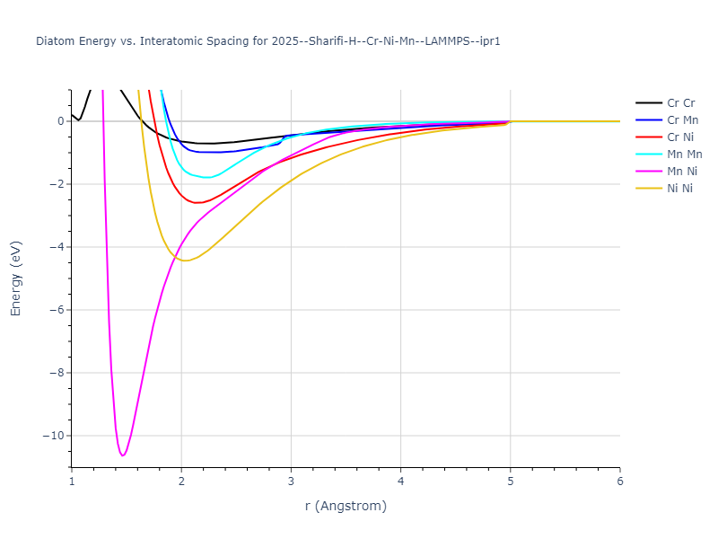
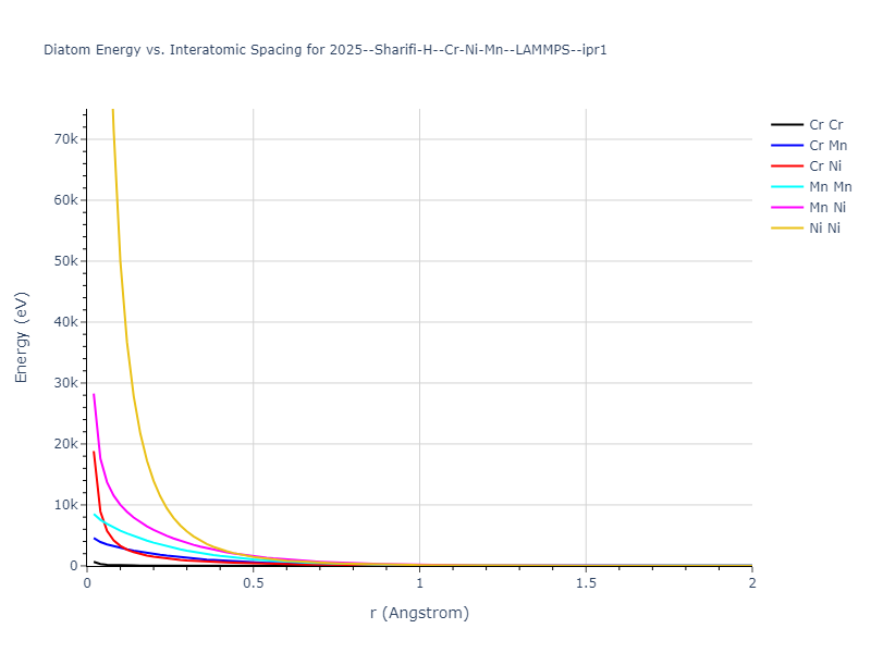
Diatom Energy vs. Interatomic Spacing
Plots of the potential energy vs interatomic spacing, r, are shown below for all diatom sets associated with the interatomic potential. This calculation provides insights into the functional form of the potential's two-body interactions. A system consisting of only two atoms is created, and the potential energy is evaluated for the atoms separated by 0.02 Å <= r <= 6.0> Å in intervals of 0.02 Å. Two plots are shown: one for the "standard" interaction distance range, and one for small values of r. The small r plot is useful for determining whether the potential is suitable for radiation studies.
The calculation method used is available as the iprPy diatom_scan calculation method.
Clicking on the image of a plot will open an interactive version of it in a new tab. The underlying data for the plots can be downloaded by clicking on the links above each plot.
Notes and Disclaimers:
- These values are meant to be guidelines for comparing potentials, not the absolute values for any potential's properties. Values listed here may change if the calculation methods are updated due to improvements/corrections. Variations in the values may occur for variations in calculation methods, simulation software and implementations of the interatomic potentials.
- As this calculation only involves two atoms, it neglects any multi-body interactions that may be important in molecules, liquids and crystals.
- NIST disclaimer
Version Information:
- 2019-11-14. Maximum value range on the shortrange plots are now limited to "expected" levels as details are otherwise lost.
- 2019-08-07. Plots added.
Click on plot to load interactive version
Click on plot to load interactive version
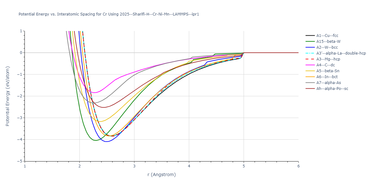
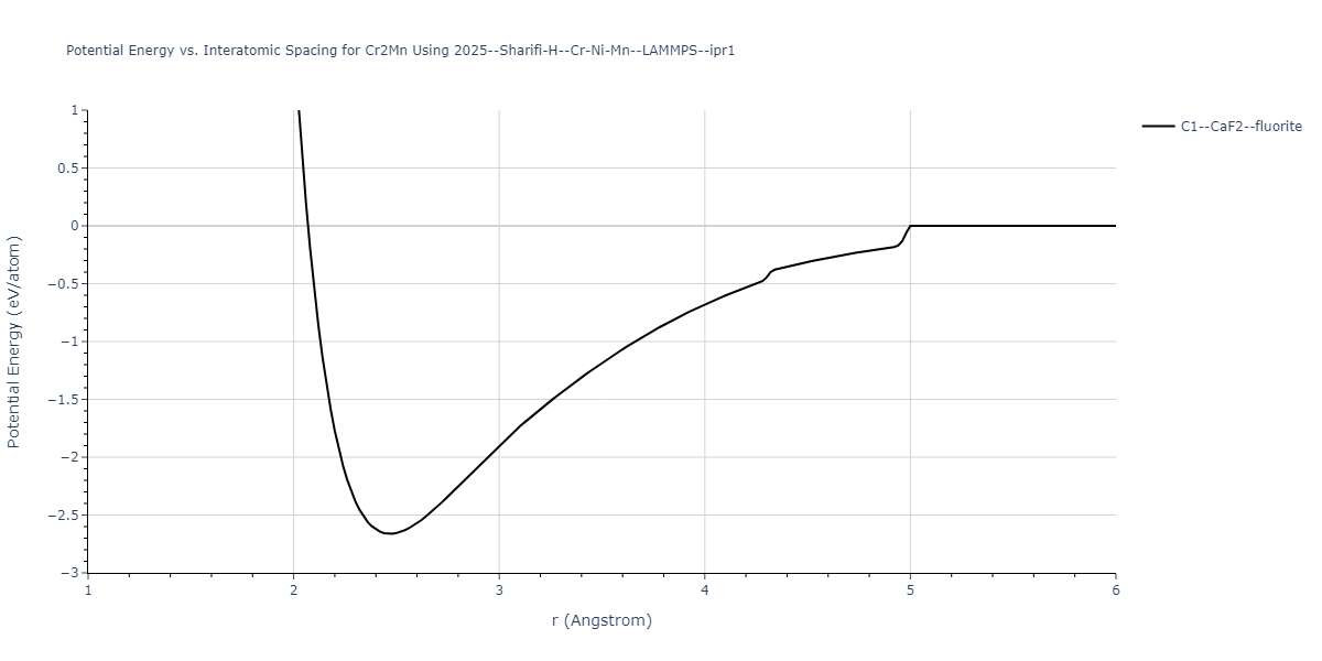
Cohesive Energy vs. Interatomic Spacing
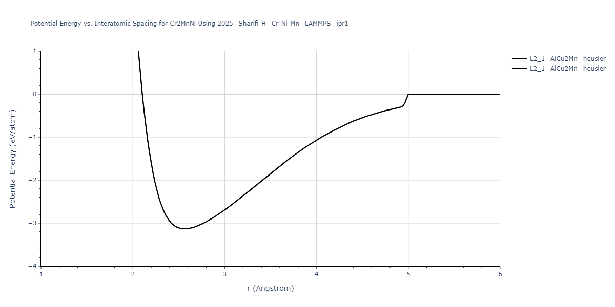
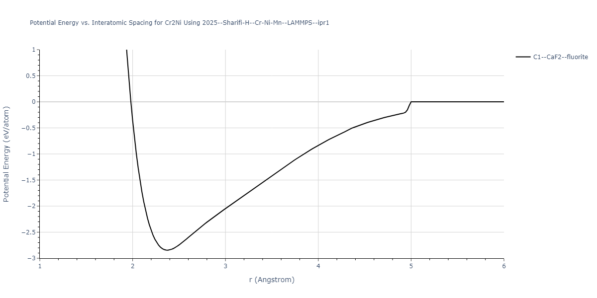
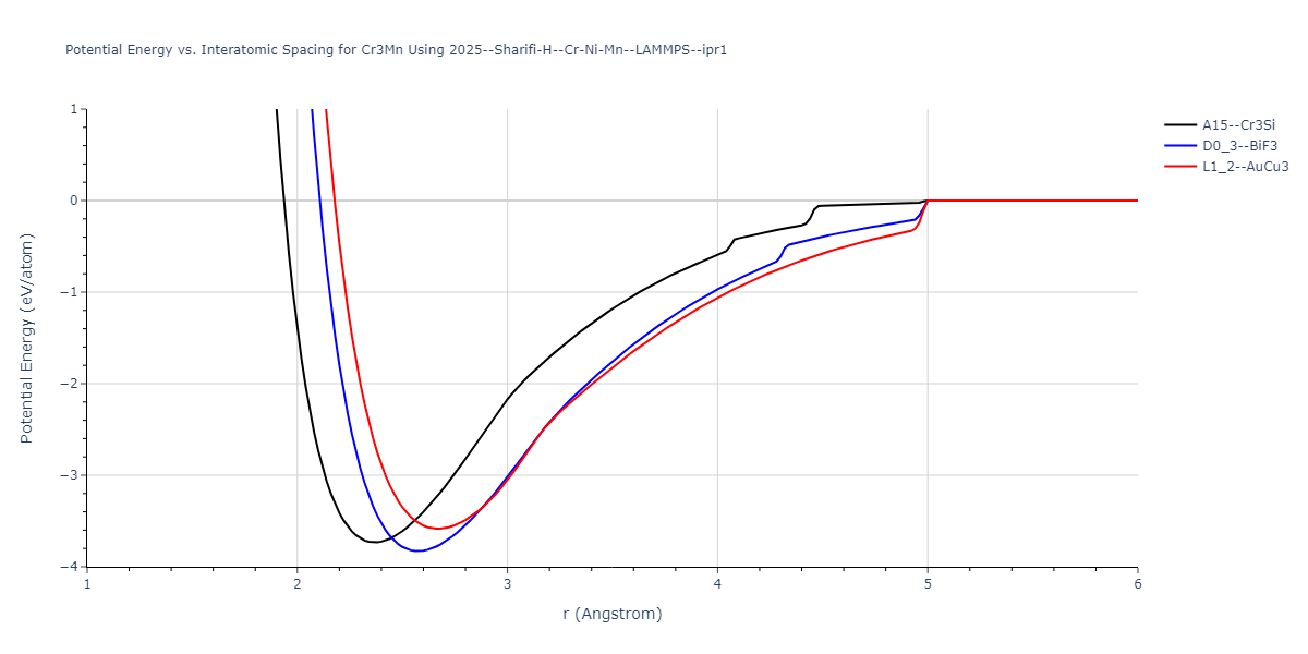
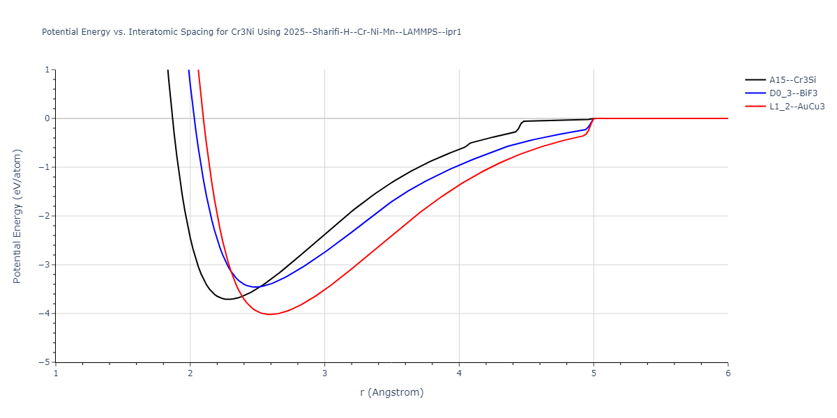
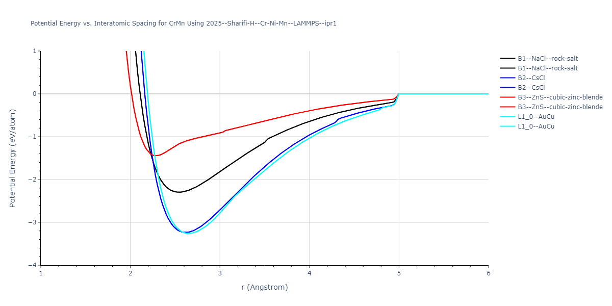
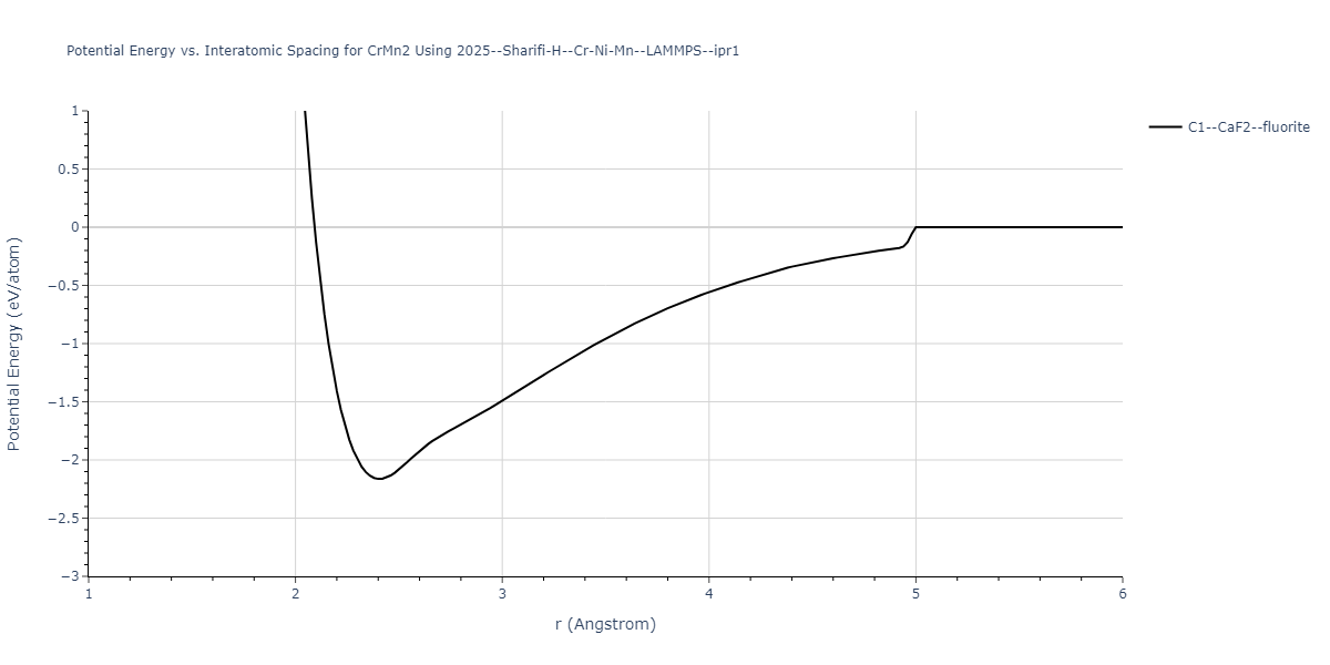
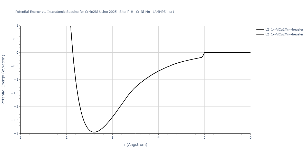
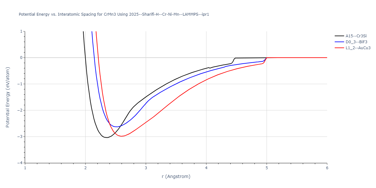
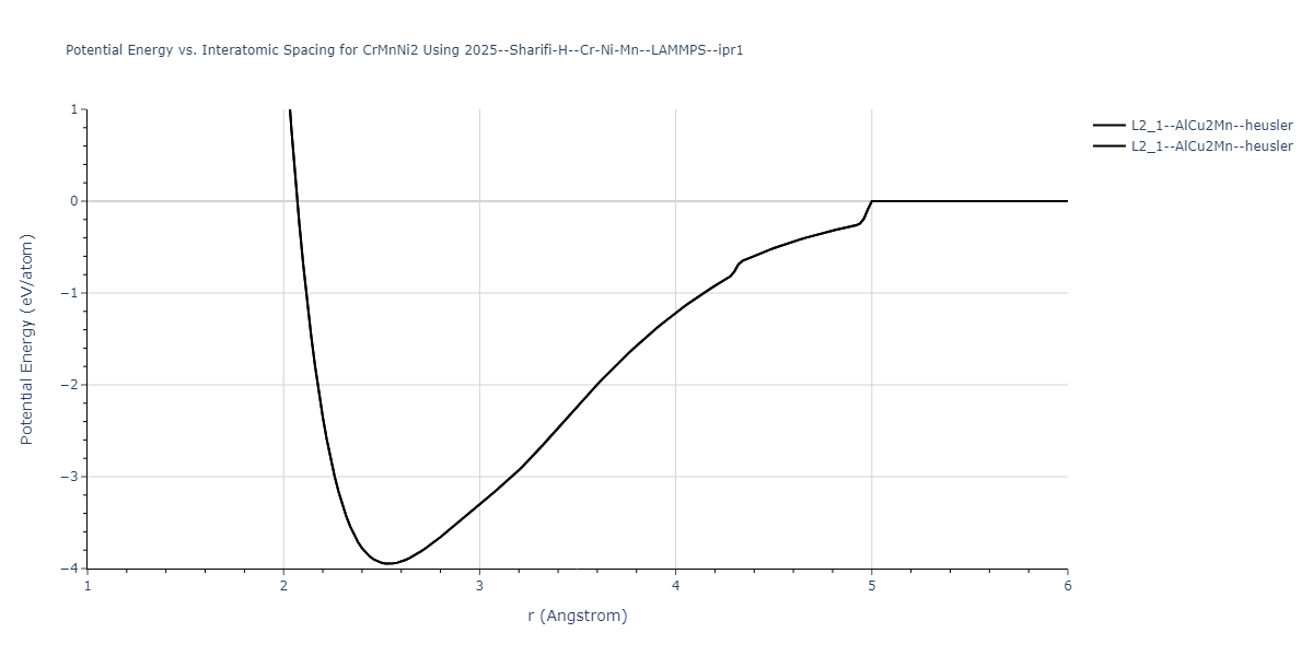
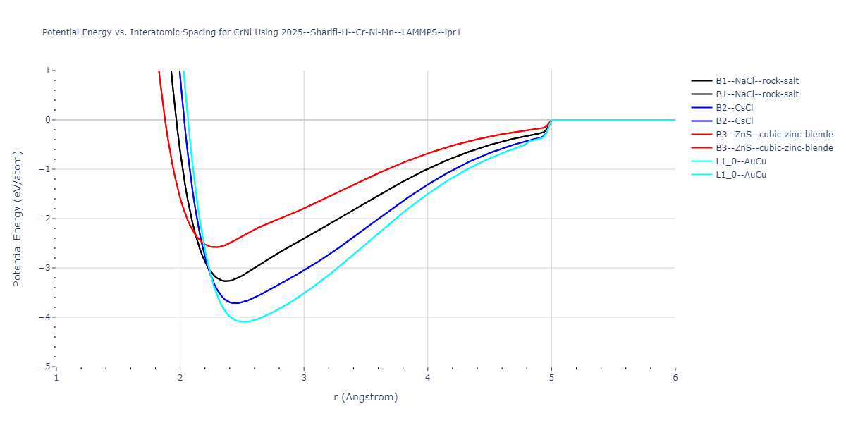
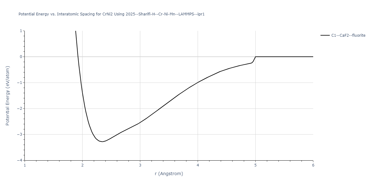
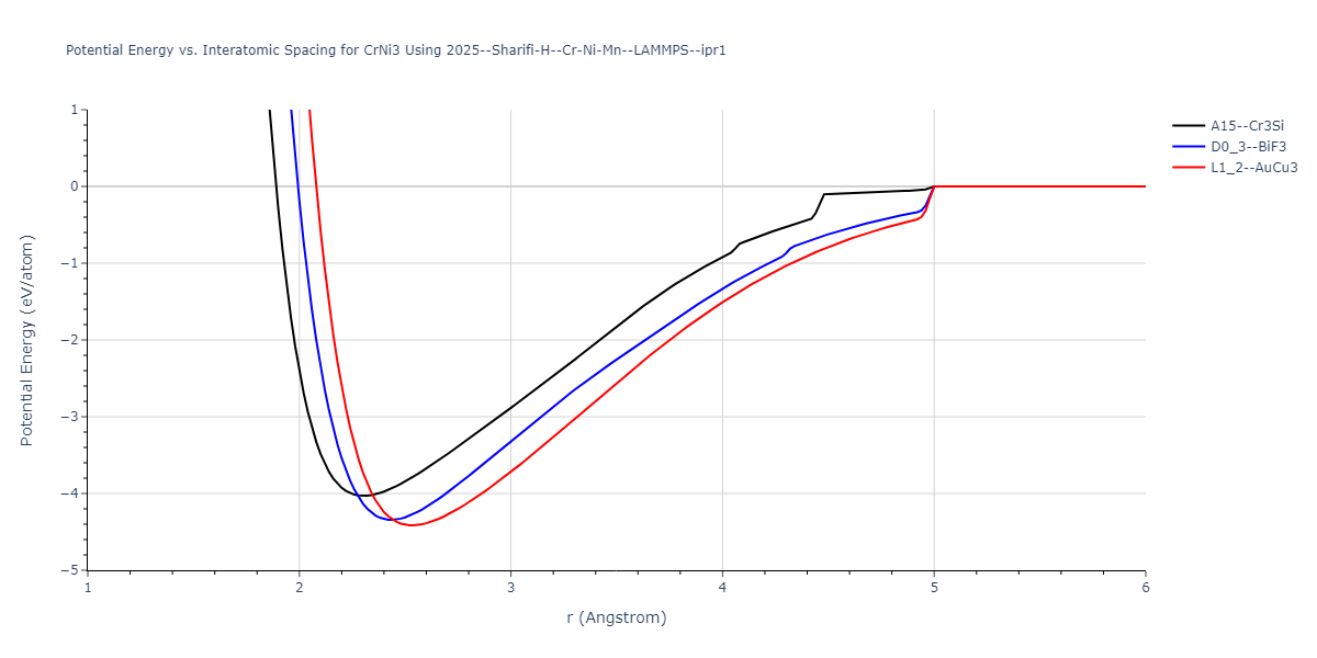
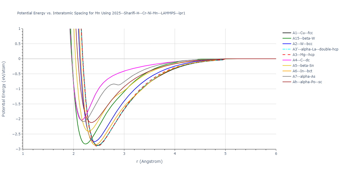
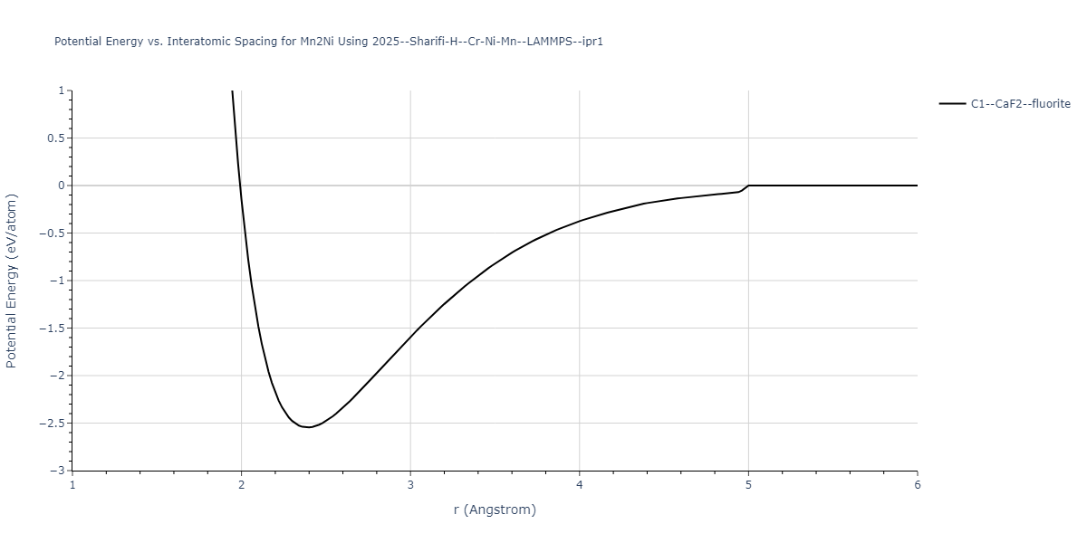
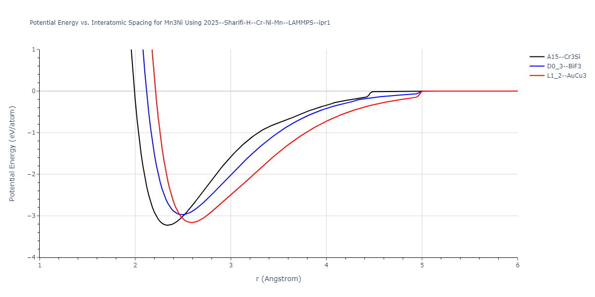
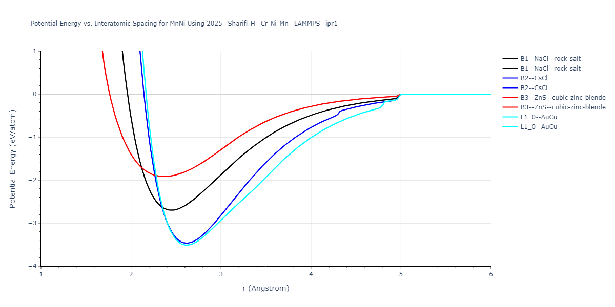
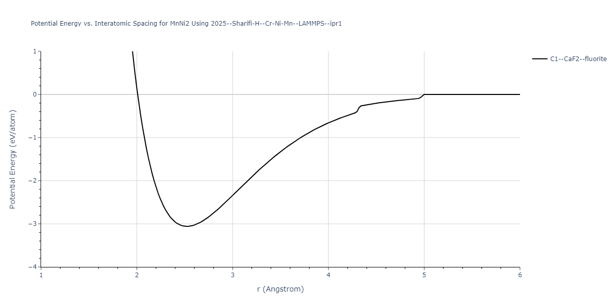
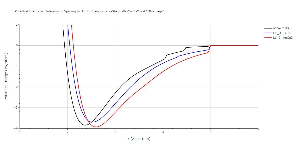
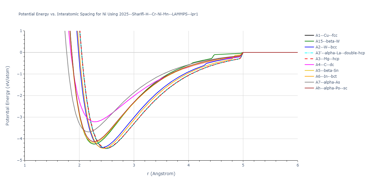
Plots of potential energy vs interatomic spacing, r, are shown below for a number of crystal structures. The structures are generated based on the ideal atomic positions and b/a and c/a lattice parameter ratios for a given crystal prototype. The size of the system is then uniformly scaled, and the energy calculated without relaxing the system. To obtain these plots, values of r are evaluated every 0.02 Å up to 6 Å.
The calculation method used is available as the iprPy E_vs_r_scan calculation method.
Clicking on the image of a plot will open an interactive version of it in a new tab. The underlying data for the plots can be downloaded by clicking on the links above each plot.
Notes and Disclaimers:
- These values are meant to be guidelines for comparing potentials, not the absolute values for any potential's properties. Values listed here may change if the calculation methods are updated due to improvements/corrections. Variations in the values may occur for variations in calculation methods, simulation software and implementations of the interatomic potentials.
- The minima identified by this calculation do not guarantee that the associated crystal structures will be stable since no relaxation is performed.
- NIST disclaimer
Version Information:
- 2020-12-18. Descriptions, tables and plots updated to reflect that the energy values are the measuredper atom potential energy rather than cohesive energy as some potentials have non-zero isolated atom energies.
- 2019-02-04. Values regenerated with even r spacings of 0.02 Å, and now include values less than 2 Å when possible. Updated calculation method and parameters enhance compatibility with more potential styles.
- 2019-04-26. Results for hcp, double hcp, α-As and L10 prototypes regenerated from different unit cell representations. Only α-As results show noticable (>1e-5 eV) difference due to using a different coordinate for Wykoff site c position.
- 2018-06-13. Values for MEAM potentials corrected. Dynamic versions of the plots moved to separate pages to improve page loading. Cosmetic changes to how data is shown and updates to the documentation.
- 2017-01-11. Replaced png pictures with interactive Bokeh plots. Data regenerated with 200 values of r instead of 300.
- 2016-09-28. Plots for binary structures added. Data and plots for elemental structures regenerated. Data values match the values of the previous version. Data table formatting slightly changed to increase precision and ensure spaces between large values. Composition added to plot title and structure names made longer.
- 2016-04-07. Plots for elemental structures added.
Crystal Structure Predictions
Computed lattice constants and cohesive/potential energies are displayed for a variety of crystal structures. The values displayed here are obtained using the following process.
- Initial crystal structure guesses are taken from:
- The iprPy E_vs_r_scan calculation results (shown above) by identifying all energy minima along the measured curves for a given crystal prototype + composition.
- Structures in the Materials Project and OQMD DFT databases.
- All initial guesses are relaxed using three independent methods using a 10x10x10 supercell:
- "box": The system's lattice constants are adjusted to zero pressure without internal relaxations using the iprPy relax_box calculation with a strainrange of 1e-6.
- "static": The system's lattice and atomic positions are statically relaxed using the iprPy relax_static calculation with a minimization force tolerance of 1e-10 eV/Angstrom.
- "dynamic": The system's lattice and atomic positions are dynamically relaxed for 10000 timesteps of 0.01 ps using the iprPy relax_dynamic calculation with an nph integration plus Langevin thermostat. The final configuration is then used as input in running an iprPy relax_static calculation with a minimization force tolerance of 1e-10 eV/Angstrom.
- The relaxed structures obtained from #2 are then evaluated using the spglib package to identify an ideal crystal unit cell based on the results.
- The space group information of the ideal unit cells is compared to the space group information of the corresponding reference structures to identify which structures transformed upon relaxation. The structures that did not transform to a different structure are listed in the table(s) below. The "method" field indicates the most rigorous relaxation method where the structure did not transform. The space group information is also used to match the DFT reference structures to the used prototype, where possible.
- The cohesive energy, Ecoh, is calculated from the measured potential energy per atom, Epot$, by subtracting the isolated energy averaged across all atoms in the unit cell. The isolated atom energies of each species model is obtained either by evaluating a single atom atomic configuration, or by identifying the first energy plateau from the diatom scan calculations for r > 2 Å.
The calculation methods used are implemented into iprPy as the following calculation styles
Notes and Disclaimers:
- These values are meant to be guidelines for comparing potentials, not the absolute values for any potential's properties. Values listed here may change if the calculation methods are updated due to improvements/corrections. Variations in the values may occur for variations in calculation methods, simulation software and implementations of the interatomic potentials.
- The presence of any structures in this list does not guarantee that those structures are stable. Also, the lowest energy structure may not be included in this list.
- Multiple values for the same crystal structure but different lattice constants are possible. This is because multiple energy minima are possible for a given structure and interatomic potential. Having multiple energy minima for a structure does not necessarily make the potential "bad" as unwanted configurations may be unstable or correspond to conditions that may not be relevant to the problem of interest (eg. very high strains).
- NIST disclaimer
Version Information:
- 2025-07-02. All "mp-" reference structure calculations were re-relaxed using the updated Materials Project database rather than the original database structures. Also, a bug was fixed that caused the "static" relaxations to occasionally throw unnecessary errors. This was fixed and all affected calculations were reset and performed again.
- 2022-05-27. The "box" method results have all been redone with an updated methodology more suited for non-orthogonal systems.
- 2020-12-18. Cohesive energies have been corrected by making them relative to the energies of the isolated atoms. The previous cohesive energy values are now listed as the potential energies.
- 2019-06-07. Structures with positive or near zero cohesive energies removed from the display tables. All values still present in the raw data files.
- 2019-04-26. Calculations now computed for each implementation. Results for hcp, double hcp, α-As and L10 prototypes regenerated from different unit cell representations.
- 2018-06-14. Methodology completely changed affecting how the information is displayed. Calculations involving MEAM potentials corrected.
- 2016-09-28. Values for simple compounds added. All identified energy minima for each structure are listed. The existing elemental data was regenerated. Most values are consistent with before, but some differences have been noted. Specifically, variations are seen with some values for potentials where the elastic constants don't vary smoothly near the equilibrium state. Additionally, the inclusion of some high-energy structures has changed based on new criteria for identifying when structures have relaxed to another structure.
- 2016-04-07. Values for elemental crystal structures added. Only values for the global energy minimum of each unique structure given.
Download raw data (including filtered results)
Reference structure matches:
A1--Cu--fcc = mp-8633, oqmd-592135, oqmd-1214518
A15--beta-W = mp-17, oqmd-620565, oqmd-691761, oqmd-1214963, oqmd-1280318
A2--W--bcc = mp-90, oqmd-676284, oqmd-676532, oqmd-677049, oqmd-685486, oqmd-690214, oqmd-691769, oqmd-1215141
A3'--alpha-La--double-hcp = oqmd-1215409
A3--Mg--hcp = mp-89, oqmd-592444, oqmd-622452, oqmd-1215319
A4--C--dc = oqmd-1215498
A5--beta-Sn = oqmd-1215587
A6--In--bct = oqmd-1215676
A7--alpha-As = oqmd-1215765
| prototype | method | Ecoh (eV/atom) | Epot (eV/atom) | a0 (Å) | b0 (Å) | c0 (Å) | α (degrees) | β (degrees) | γ (degrees) |
|---|---|---|---|---|---|---|---|---|---|
| A2--W--bcc | dynamic | -4.1 | -4.1 | 2.881 | 2.881 | 2.881 | 90.0 | 90.0 | 90.0 |
| A15--beta-W | dynamic | -4.0458 | -4.0458 | 4.5939 | 4.5939 | 4.5939 | 90.0 | 90.0 | 90.0 |
| oqmd-1214785 | static | -3.9767 | -3.9767 | 8.9092 | 8.9092 | 8.9092 | 90.0 | 90.0 | 90.0 |
| oqmd-1214785 | box | -3.9723 | -3.9723 | 8.9099 | 8.9099 | 8.9099 | 90.0 | 90.0 | 90.0 |
| oqmd-1214874 | dynamic | -3.9683 | -3.9683 | 6.2422 | 6.2422 | 6.2422 | 90.0 | 90.0 | 90.0 |
| oqmd-691775 | dynamic | -3.9539 | -3.9539 | 2.6333 | 2.6333 | 6.0702 | 90.0 | 90.0 | 120.0 |
| oqmd-1214874 | box | -3.9505 | -3.9505 | 6.2466 | 6.2466 | 6.2466 | 90.0 | 90.0 | 90.0 |
| mp-1192789 | dynamic | -3.9289 | -3.9289 | 8.6337 | 8.6337 | 4.6672 | 90.0 | 90.0 | 90.0 |
| mp-1192789 | box | -3.9216 | -3.9216 | 8.6703 | 8.6703 | 4.6358 | 90.0 | 90.0 | 90.0 |
| oqmd-631035 | box | -3.9213 | -3.9213 | 8.605 | 8.605 | 4.6901 | 90.0 | 90.0 | 90.0 |
| A3--Mg--hcp | box | -3.8551 | -3.8551 | 2.5958 | 2.5958 | 4.176 | 90.0 | 90.0 | 120.0 |
| A3--Mg--hcp | box | -3.8551 | -3.8551 | 2.5958 | 2.5958 | 4.176 | 90.0 | 90.0 | 120.0 |
| oqmd-1216032 | box | -3.8496 | -3.8496 | 2.5917 | 2.5917 | 18.8615 | 90.0 | 90.0 | 120.0 |
| A3'--alpha-La--double-hcp | box | -3.8472 | -3.8472 | 2.5898 | 2.5898 | 8.3968 | 90.0 | 90.0 | 120.0 |
| A6--In--bct | static | -3.8397 | -3.8397 | 2.5633 | 2.5633 | 3.7142 | 90.0 | 90.0 | 90.0 |
| A1--Cu--fcc | static | -3.8396 | -3.8396 | 3.6546 | 3.6546 | 3.6546 | 90.0 | 90.0 | 90.0 |
| A7--alpha-As | box | -3.8394 | -3.8394 | 2.5842 | 2.5842 | 12.6606 | 90.0 | 90.0 | 120.0 |
| mp-1059289 | box | -3.828 | -3.828 | 2.522 | 4.5755 | 4.2352 | 90.0 | 90.0 | 90.0 |
| oqmd-1214696 | box | -3.556 | -3.556 | 2.7658 | 4.1065 | 8.9436 | 90.0 | 90.0 | 90.0 |
| oqmd-1215052 | box | -3.5332 | -3.5332 | 4.1071 | 8.9396 | 2.7601 | 90.0 | 90.0 | 90.0 |
| A5--beta-Sn | static | -3.1733 | -3.1733 | 4.6024 | 4.6024 | 2.4886 | 90.0 | 90.0 | 90.0 |
| oqmd-1215943 | box | -2.7125 | -2.7125 | 4.02 | 4.02 | 4.0871 | 90.0 | 90.0 | 120.0 |
| Ah--alpha-Po--sc | static | -2.5234 | -2.5234 | 2.4401 | 2.4401 | 2.4401 | 90.0 | 90.0 | 90.0 |
| A7--alpha-As | box | -2.3174 | -2.3174 | 3.392 | 3.392 | 9.2715 | 90.0 | 90.0 | 120.0 |
| A4--C--dc | box | -1.8425 | -1.8425 | 5.2484 | 5.2484 | 5.2484 | 90.0 | 90.0 | 90.0 |
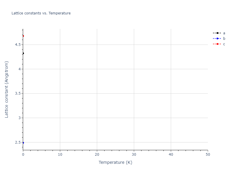
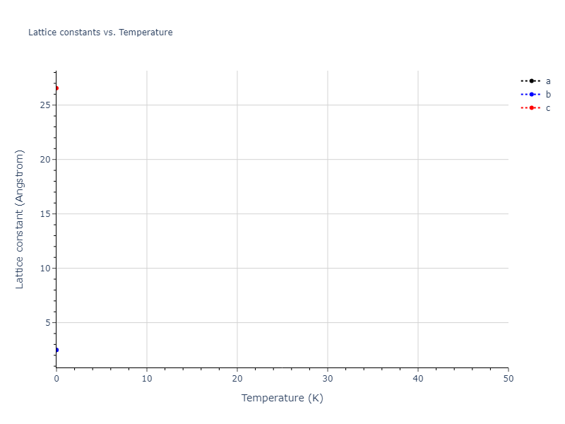
MD Solid Property Predictions
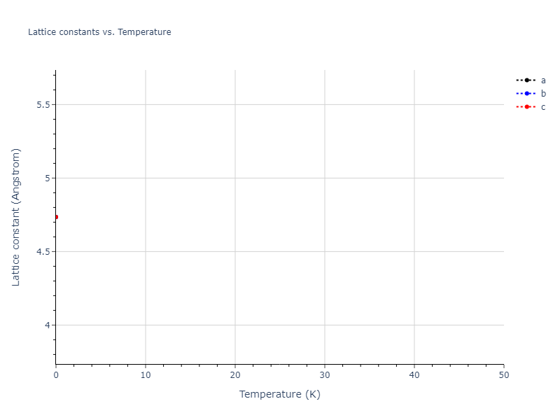
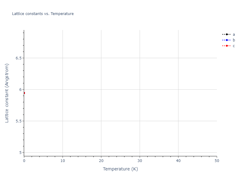
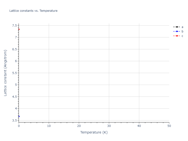
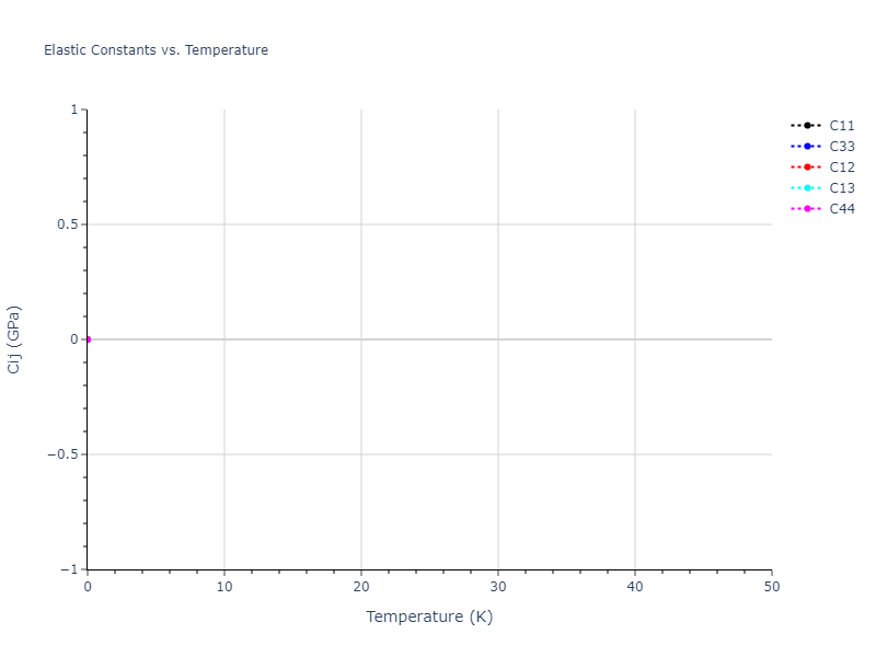
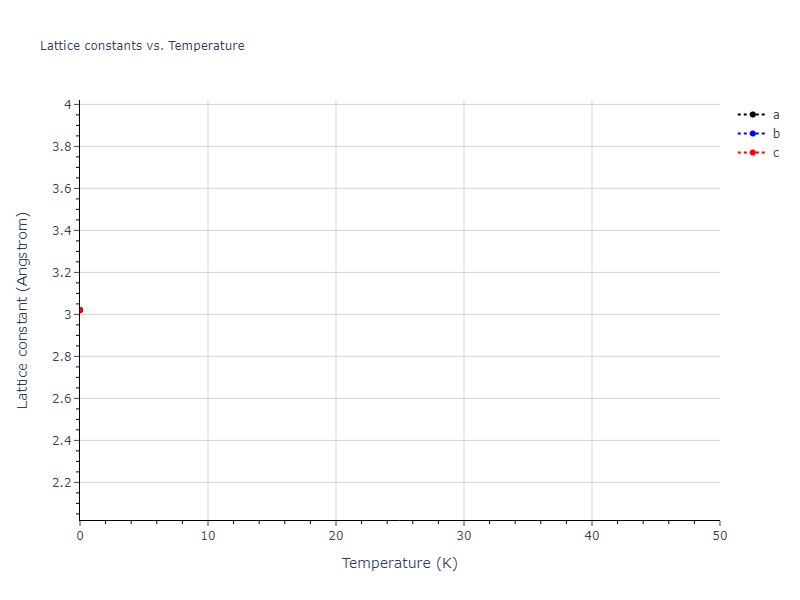
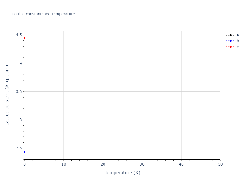
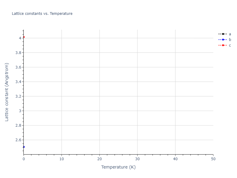
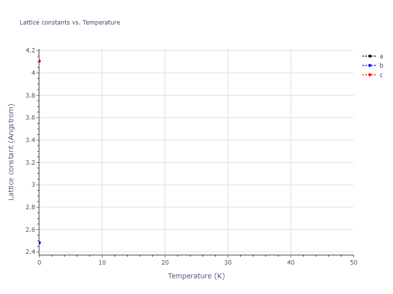
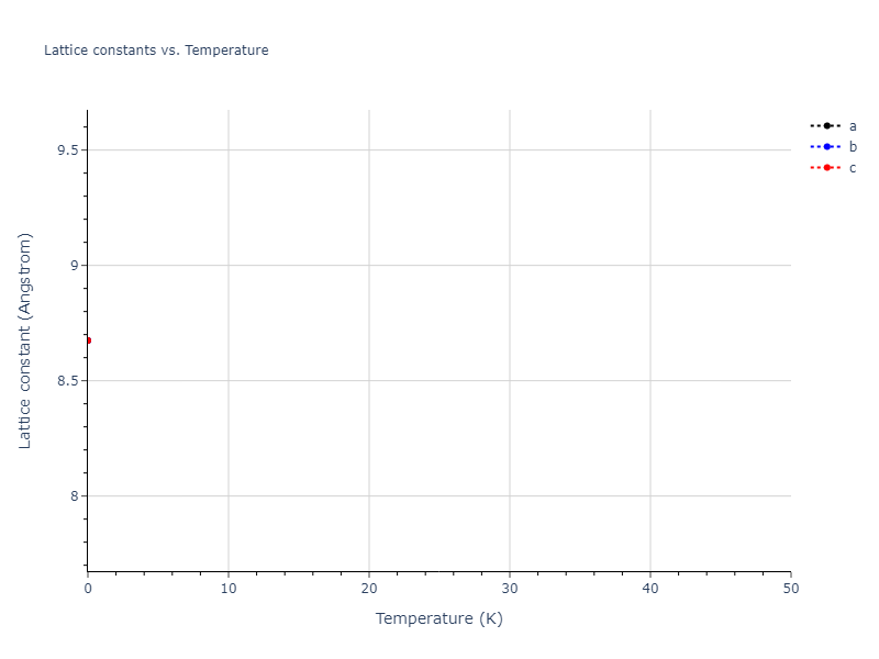
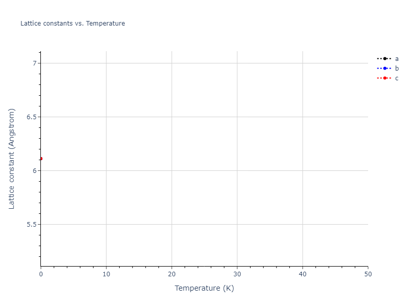
Plots of lattice and elastic constants are shown as a function of temperature. The 0K points were taken from the Crystal Structure Predictions and the Elastic Constants Predictions sections above for the unique crystal structures relaxed with the "dynamic" method. Starting from the 0 K relaxed crystal unit cells, supercell systems are created by replicating all three dimensions by the same multiplier to achieve at least 4000 atoms. The systems are then relaxed at 50 K and zero pressure using 1 million NPT steps. Lattice constants are estimated by averaging the measured box dimensions. Temperatures are iteratively increased by 50 K, with each subsequent relaxation calculation starting from the final atomic configuration at the previous temperature and relaxing for another 1 million steps.
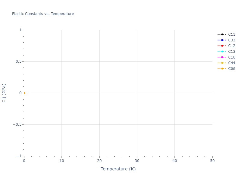
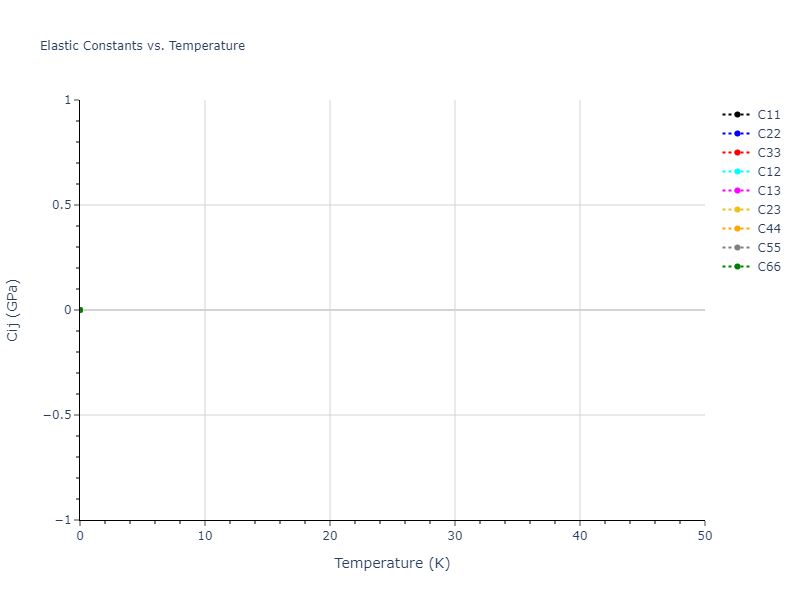
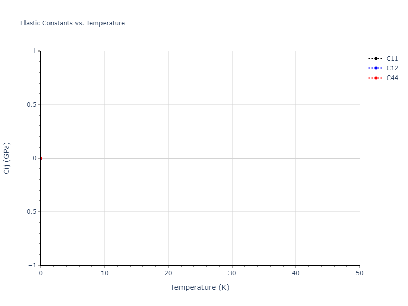
The elastic constants are calculated using the deformation–fluctuation hybrid method. Starting from the final atomic configurations of the dynamic relaxations, the system is allowed to evolve at constant volume with a Langevin thermostat. The Born matrix is computed during this run by evaluating how the atomic forces would vary due to applied linear strain fields. The elastic constants can then be estimated using the averaged Born matrix values and the averaged stresses on the system.
The calculation methods used are available as the iprPy relax_dynamic and elastic_constants_dynamic calculation methods.
Clicking on the image of a plot will open an interactive version of it in a new tab. The underlying data for the plots can be downloaded by clicking on the links above each plot.
Notes and Disclaimers:
- The maximum temperature shown for a crystal either corresponds to the maximum value that has been computed so far, or the maximum value that the structure is believed to have remained untransformed. The unstable/transformation temperature identification is mostly automated and can miss transitions not associated with large discontinuities in property values with changing temperature.
- For succinctness, the elastic constants displayed here are averaged according to the 0 K structure's crystal symmetry family. If the structures deviate from the expected symmetry at higher temperatures, the values may not be valid. Raw results are available for verification if requested.
- NIST disclaimer
Version Information:
- 2025-08-07. Plots added.
Click on plot to load interactive version

Click on plot to load interactive version


MD Thermodynamic Predictions
Plots of internal energy, Gibbs free energy, entropy, heat capacity and volume are shown here as a function of temperature for various crystal structures and liquid phases. The included crystal structures correspond to those in the Solid Structures vs. Temperature section, and the liquid phases to those in the Liquid Properties section. Internal energy and volume are taken from the associated structure relaxations mentioned in those previous sections. Constant pressure heat capacity is estimated using 3-point numerical derivatives of enthalpy versus temperature. Note that since all simulations done here are at 0 pressure, internal energy and enthalpy are equivalent.
The Gibbs energies of the phases are estimated using thermodynamic integration between the interatomic potential in question and a simpler model with known Gibbs free energy values. For solids, the reference model is an Einstein solid, while for liquids it is the Uhlenbeck-Ford potential. Besides a short run at the start of the solid calculations to estimate Einstein model spring constants, the two calculations proceed similarly. Starting with the final relaxation configurations, the systems are stabilized for 25,000 steps. Then, over the next 50,000 steps the potential is swapped out for the reference potential. The system is then stabilized for another 25,000 steps with the reference model before a reverse swap of 50,000 steps is performed. The simulation ends with one final 25,000 step stabilization period. From the simulation, the irreversible work of transformation is estimated and used to compute the absolute Gibbs free energy of the target phase and potential relative to the reference potential. Entropy is estimated as the difference in enthalpy and Gibbs free energy and divided by temperature.
The calculation methods used are available as the iprPy relax_dynamic, relax_liquid_redo, free_energy, and free_energy_liquid calculation methods.
Clicking on the image of a plot will open an interactive version of it in a new tab. The underlying data for the plots can be downloaded by clicking on the links above each plot.
Notes and Disclaimers:
- Good free energy estimates require that the initial and final phases before and after the thermodynamic integration remain the same. This is not an issue with the liquid calculations as the Uhlenbeck-Ford model always predicts a liquid, but may be an issue for the solid phase estimates. This is likely to be an issue for non-compact phases which the Einstein model is poor at representing.
- NIST disclaimer
Version Information:
- 2025-08-07. Plots added.