 FiPy
FiPyDesign and Implementation
The goal of FiPy is to provide a highly customizable, open source code for modeling problems involving coupled sets of PDEs. FiPy allows users to select and customize modules from within the framework. FiPy has been developed to address model problems in materials science such as poly-crystals, dendritic growth and electrochemical deposition. These applications all contain various combinations of PDEs with differing forms in conjunction with other unusual physics (over varying length scales) and unique solution procedures. The philosophy of FiPy is to enable customization while providing a library of efficient modules for common objects and data types.
Design
Numerical Approach
The solution algorithms given in the FiPy examples involve combining sets of PDEs while tracking an interface where the parameters of the problem change rapidly. The phase field method and the level set method are specialized techniques to handle the solution of PDEs in conjunction with a deforming interface. FiPy contains several examples of both methods.
FiPy uses the well-known Finite Volume Method (FVM) to reduce the model equations to a form tractable to linear solvers.
Object Oriented Structure
FiPy is programmed in an object-oriented manner. The benefit of object oriented programming mainly lies in encapsulation and inheritance. Encapsulation refers to the tight integration between certain pieces of data and methods that act on that data. Encapsulation allows parts of the code to be separated into clearly defined independent modules that can be re-applied or extended in new ways. Inheritance allows code to be reused, overridden, and new capabilities to be added without altering the original code. An object is treated by its users as an abstraction; the details of its implementation and behavior are internal.
Test Based Development
FiPy has been developed with a large number of test cases. These test cases are in two categories. The lower level tests operate on the core modules at the individual method level. The aim is that every method within the core installation has a test case. The high level test cases operate in conjunction with example solutions and serve to test global solution algorithms and the interaction of various modules.
With this two-tiered battery of tests, at any stage in code development, the test cases can be executed and errors can be identified. A comprehensive test base provides reassurance that any code breakages will be clearly demonstrated with a broken test case. A test base also aids dissemination of the code by providing simple examples and knowledge of whether the code is working on a particular computer environment.
Open Source
In recent years, there has been a movement to release software under open source and associated unrestricted licenses, especially within the scientific community. These licensing terms allow users to develop their own applications with complete access to the source code and then either contribute back to the main source repository or freely distribute their new adapted version.
As a product of the National Institute of Standards and Technology, the FiPy framework is placed in the public domain as a matter of U. S. Federal law. Furthermore, FiPy is built upon existing open source tools. Others are free to use FiPy as they see fit and we welcome contributions to make FiPy better.
High-Level Scripting Language
Programming languages can be broadly lumped into two categories: compiled languages and interpreted (or scripting) languages. Compiled languages are converted from a human-readable text source file to a machine-readable binary application file by a sequence of operations generally referred to as “compiling” and “linking.” The binary application can then be run as many times as desired, but changes will provoke a new cycle of compiling and linking. Interpreted languages are converted from human-readable to machine-readable on the fly, each time the script is executed. Because the conversion happens every time [1], interpreted code is usually slower when running than compiled code. On the other hand, code development and debugging tends to be much easier and fluid when it’s not necessary to wait for compile and link cycles after every change. Furthermore, because the conversion happens in real time, it is possible to have interactive sessions in a scripting language that are not generally possible in compiled languages.
Another distinction, somewhat orthogonal, but closely related, to that between compiled and interpreted languages, is between low-level languages and high-level languages. Low-level languages describe actions in simple terms that are closer to the way the computer actually functions. High-level languages describe actions in more complex and abstract terms that are closer to the way the programmer thinks about the problem at hand. This increased complexity in the meaning of an expression renders simpler code, because the details of the implementation are hidden away in the language internals or in an external library. For example, a low-level matrix multiplication written in C might be rendered as
if (Acols != Brows)
    error "these matrix shapes cannot be multiplied";

C = (float *) malloc(sizeof(float) * Bcols * Arows);

for (i = 0; i < Bcols; i++) {
    for (j = 0; j < Arows; j++) {
        C[i][j] = 0;
        for (k = 0; k < Acols; k++) {
            C[i][j] += A[i][k] * B[k][j];
        }
    }
}
Note that the dimensions of the arrays must be supplied externally, as C provides no intrinsic mechanism for determining the shape of an array. An equivalent high-level construction might be as simple as
C = A * B
All of the error checking, dimension measuring, and space allocation
is handled automatically by low-level code that is intrinsic to the
high-level matrix multiplication operator. The high-level code
“knows” that matrices are involved, how to get their shapes, and to
interpret “*” as a matrix multiplier instead of an arithmetic
one. All of this allows the programmer to think about the operation
of interest and not worry about introducing bugs in low-level code
that is not unique to their application.
Although it needn’t be true, for a variety of reasons, compiled languages tend to be low-level and interpreted languages tend to be high-level. Because low-level languages operate closer to the intrinsic “machine language” of the computer, they tend to be faster at running a given task than high-level languages, but programs written in them take longer to write and debug. Because running performance is a paramount concern, most scientific codes are written in low-level compiled languages like FORTRAN or C.
A rather common scenario in the development of scientific codes is
that the first draft hard-codes all of the problem parameters. After
a few (hundred) iterations of recompiling and relinking the
application to explore changes to the parameters, code is added to
read an input file containing a list of numbers. Eventually, the
point is reached where it is impossible to remember which parameter
comes in which order or what physical units are required, so code is
added to, for example, interpret a line beginning with “#” as a
comment. At this point, the scientist has begun developing a
scripting language without even knowing it. Unfortunately for them,
very few scientists have actually studied computer science or actually
know anything about the design and implementation of script
interpreters. Even if they have the expertise, the time spent
developing such a language interpreter is time not spent actually
doing research.
In contrast, a number of very powerful scripting languages, such as Tcl, Java, Python, Ruby, and even the venerable BASIC, have open source interpreters that can be embedded directly in an application, giving scientific codes immediate access to a high-level scripting language designed by someone who actually knew what they were doing.
We have chosen to go a step further and not just embed a full-fledged scripting language in the FiPy framework, but instead to design the framework from the ground up in a scripting language. While runtime performance is unquestionably important, many scientific codes are run relatively little, in proportion to the time spent developing them. If a code can be developed in a day instead of a month, it may not matter if it takes another day to run instead of an hour. Furthermore, there are a variety of mechanisms for diagnosing and optimizing those portions of a code that are actually time-critical, rather than attempting to optimize all of it by using a language that is more palatable to the computer than to the programmer. Thus FiPy, rather than taking the approach of writing the fast numerical code first and then dealing with the issue of user interaction, initially implements most modules in high-level scripting language and only translates to low-level compiled code those portions that prove inefficient [2].
Python Programming Language
Acknowledging that several scripting languages offer a number, if not all, of the features described above, we have selected Python for the implementation of FiPy. Python is
an interpreted language that combines remarkable power with very clear syntax,
freely usable and distributable, even for commercial use,
fully object oriented,
distributed with powerful automated testing tools (
doctest,unittest),actively used and extended by other scientists and mathematicians (SciPy, NumPy, ScientificPython, Pysparse).
easily integrated with low-level languages such as C (
weave,blitz, PyRex).
Implementation
The Python classes that make up FiPy are described in detail in
fipy Package Documentation, but we give a brief overview here. FiPy is
based around three fundamental Python classes:
Mesh,
Variable, and
Term. Using the terminology of
Theoretical and Numerical Background:
- A
Meshobject represents the domain of interest. FiPy contains many different specific mesh classes to describe different geometries.
- A
Variableobject represents a quantity or field that can change during the problem evolution. A particular type of
Variable, called aCellVariable, represents at the centers of the cells of the
Mesh. ACellVariabledescribes the values of the field, but it is not concerned with their geometry;
that role is taken by the Mesh.An important property of
Variableobjects is that they can describe dependency relationships, such that:>>> a = Variable(value = 3) >>> b = a * 4
does not assign the value
12tob, but rather it assigns a multiplication operator object tob, which depends on theVariableobjecta:>>> b (Variable(value = 3) * 4) >>> a.setValue(5) >>> b (Variable(value = 5) * 4)
The numerical value of the
Variableis not calculated until it is needed (a process known as “lazy evaluation”):>>> print b 20
- A
Termobject represents any of the terms in Equation (2) or any linear combination of such terms. Early in the development of FiPy, a distinction was made between
Equationobjects, which represented all of Equation (2), andTermobjects, which represented the individual terms in that equation. TheEquationobject has since been eliminated as redundant.Termobjects can be single entities such as aDiffusionTermor a linear combination of otherTermobjects that build up to form an expression such as Equation (2).
Beyond these three fundamental classes of Mesh,
Variable, and Term, FiPy is composed of a
number of related classes.
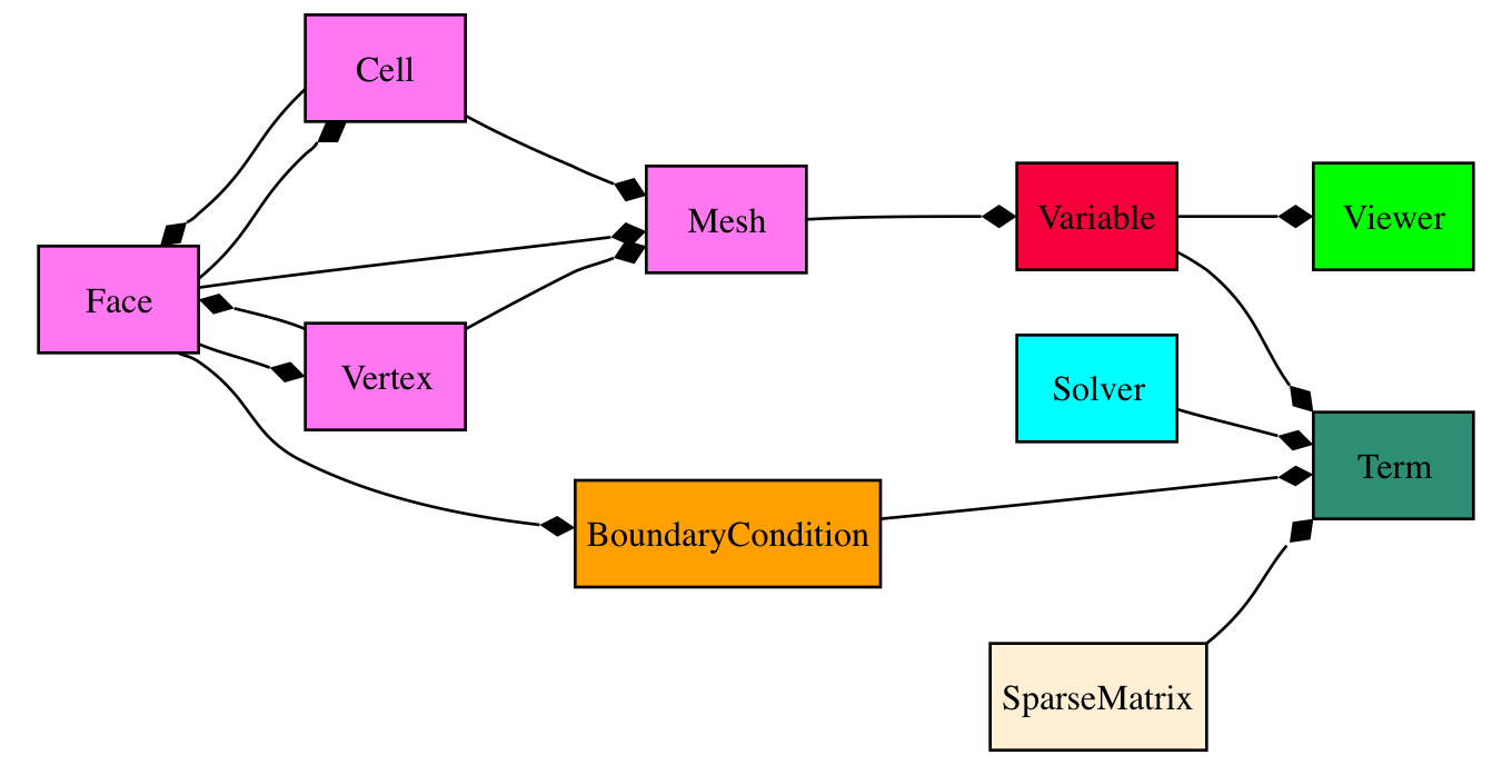
Primary object relationships in FiPy.
A Mesh object is composed of cells. Each cell is
defined by its bounding faces and each face is defined by its bounding
vertices. A Term object encapsulates the
contributions to the _SparseMatrix that
defines the solution of an equation.
BoundaryCondition
objects are used to describe the conditions on the boundaries of the
Mesh, and each
Term interprets the BoundaryCondition
objects as necessary to modify the
_SparseMatrix. An equation constructed
from Term objects can apply a unique
Solver to invert its
_SparseMatrix in the most expedient and
stable fashion. At any point during the solution, a Viewer can be invoked to display the values of
the solved Variable objects.
At this point, it will be useful to examine some of the example problems in Examples. More classes are introduced in the examples, along with illustrations of their instantiation and use.
Footnotes