examples.phase.anisotropy¶

Solve a dendritic solidification problem.

To convert a liquid material to a solid, it must be cooled to a temperature below its melting point (known as “undercooling” or “supercooling”). The rate of solidification is often assumed (and experimentally found) to be proportional to the undercooling. Under the right circumstances, the solidification front can become unstable, leading to dendritic patterns. Warren, Kobayashi, Lobkovsky and Carter [13] have described a phase field model (“Allen-Cahn”, “non-conserved Ginsberg-Landau”, or “model A” of Hohenberg & Halperin) of such a system, including the effects of discrete crystalline orientations (anisotropy).

We start with a regular 2D Cartesian mesh

>>> from fipy import Variable, CellVariable, Grid2D, TransientTerm, DiffusionTerm, ImplicitSourceTerm, Viewer, Matplotlib2DGridViewer
>>> from fipy.tools import numerix
>>> dx = dy = 0.025
>>> if __name__ == '__main__':
...     nx = ny = 500
... else:
...     nx = ny = 20
>>> mesh = Grid2D(dx=dx, dy=dy, nx=nx, ny=ny)

and we’ll take fixed timesteps

>>> dt = 5e-4

We consider the simultaneous evolution of a “phase field” variable $\phi$ (taken to be 0 in the liquid phase and 1 in the solid)

>>> phase = CellVariable(name=r'$\phi$', mesh=mesh, hasOld=True)

and a dimensionless undercooling $\Delta T$ ( $\Delta T = 0$ at the melting point)

>>> dT = CellVariable(name=r'$\Delta T$', mesh=mesh, hasOld=True)

The hasOld flag causes the storage of the value of variable from the previous timestep. This is necessary for solving equations with non-linear coefficients or for coupling between PDEs.

The governing equation for the temperature field is the heat flux equation, with a source due to the latent heat of solidification

$\frac{\partial \Delta T}{\partial t} = D_T \nabla^2 \Delta T + \frac{\partial \phi}{\partial t}$

>>> DT = 2.25
>>> heatEq = (TransientTerm()
...           == DiffusionTerm(DT)
...           + (phase - phase.old) / dt)

The governing equation for the phase field is

$\tau_{\phi} \frac{\partial \phi}{\partial t} = \nabla \cdot \mathsf{D} \nabla \phi + \phi ( 1 - \phi ) m ( \phi , \Delta T)$

where

$m(\phi, \Delta T) = \phi - \frac{1}{2} - \frac{ \kappa_1 }{ \pi } \arctan \left( \kappa_2 \Delta T \right)$

represents a source of anisotropy. The coefficient $\mathsf{D}$ is an anisotropic diffusion tensor in two dimensions

$\mathsf{D} = \alpha^2 \left( 1 + c \beta \right) \left[ \begin{matrix} 1 + c \beta & -c \frac{\partial \beta}{\partial \psi} \\ c \frac{\partial \beta}{\partial \psi} & 1 + c \beta \end{matrix} \right]$

where $\beta = \frac{ 1 - \Phi^2 } { 1 + \Phi^2}$ , $\Phi = \tan \left( \frac{ N } { 2 } \psi \right)$ , $\psi = \theta + \arctan \frac{\partial \phi / \partial y}{\partial \phi / \partial x}$ , $\theta$ is the orientation, and $N$ is the symmetry.

>>> alpha = 0.015
>>> c = 0.02
>>> N = 6.
>>> theta = numerix.pi / 8.
>>> psi = theta + numerix.arctan2(phase.faceGrad[1],
...                               phase.faceGrad[0])
>>> Phi = numerix.tan(N * psi / 2)
>>> PhiSq = Phi**2
>>> beta = (1. - PhiSq) / (1. + PhiSq)
>>> DbetaDpsi = -N * 2 * Phi / (1 + PhiSq)
>>> Ddia = (1.+ c * beta)
>>> Doff = c * DbetaDpsi
>>> I0 = Variable(value=((1, 0), (0, 1)))
>>> I1 = Variable(value=((0, -1), (1, 0)))
>>> D = alpha**2 * (1.+ c * beta) * (Ddia * I0 + Doff * I1)

With these expressions defined, we can construct the phase field equation as

>>> tau = 3e-4
>>> kappa1 = 0.9
>>> kappa2 = 20.
>>> phaseEq = (TransientTerm(tau)
...            == DiffusionTerm(D)
...            + ImplicitSourceTerm((phase - 0.5 - kappa1 / numerix.pi * numerix.arctan(kappa2 * dT))
...                                 * (1 - phase)))

We seed a circular solidified region in the center

>>> radius = dx * 5.
>>> C = (nx * dx / 2, ny * dy / 2)
>>> x, y = mesh.cellCenters
>>> phase.setValue(1., where=((x - C[0])**2 + (y - C[1])**2) < radius**2)

and quench the entire simulation domain below the melting point

>>> dT.setValue(-0.5)

In a real solidification process, dendritic branching is induced by small thermal fluctuations along an otherwise smooth surface, but the granularity of the Mesh is enough “noise” in this case, so we don’t need to explicitly introduce randomness, the way we did in the Cahn-Hilliard problem.

FiPy’s viewers are utilitarian, striving to let the user see something, regardless of their operating system or installed packages, so you won’t be able to simultaneously view two fields “out of the box”, but, because all of Python is accessible and FiPy is object oriented, it is not hard to adapt one of the existing viewers to create a specialized display:

>>> if __name__ == "__main__":
...     try:
...         import pylab
...         class DendriteViewer(Matplotlib2DGridViewer):
...             def __init__(self, phase, dT, title=None, limits={}, **kwlimits):
...                 self.phase = phase
...                 self.contour = None
...                 Matplotlib2DGridViewer.__init__(self, vars=(dT,), title=title,
...                                                 cmap=pylab.cm.hot,
...                                                 limits=limits, **kwlimits)
...
...             def _plot(self):
...                 Matplotlib2DGridViewer._plot(self)
...
...                 if self.contour is not None:
...                     for c in self.contour.collections:
...                         c.remove()
...
...                 mesh = self.phase.mesh
...                 shape = mesh.shape
...                 x, y = mesh.cellCenters
...                 z = self.phase.value
...                 x, y, z = [a.reshape(shape, order='F') for a in (x, y, z)]
...
...                 self.contour = self.axes.contour(x, y, z, (0.5,))
...
...         viewer = DendriteViewer(phase=phase, dT=dT,
...                                 title=r"%s & %s" % (phase.name, dT.name),
...                                 datamin=-0.1, datamax=0.05)
...     except ImportError:
...         viewer = MultiViewer(viewers=(Viewer(vars=phase),
...                                       Viewer(vars=dT,
...                                              datamin=-0.5,
...                                              datamax=0.5)))

and iterate the solution in time, plotting as we go,

>>> if __name__ == '__main__':
...     steps = 10000
... else:
...     steps = 10
>>> from builtins import range
>>> for i in range(steps):
...     phase.updateOld()
...     dT.updateOld()
...     phaseEq.solve(phase, dt=dt)
...     heatEq.solve(dT, dt=dt)
...     if __name__ == "__main__" and (i % 10 == 0):
...         viewer.plot()

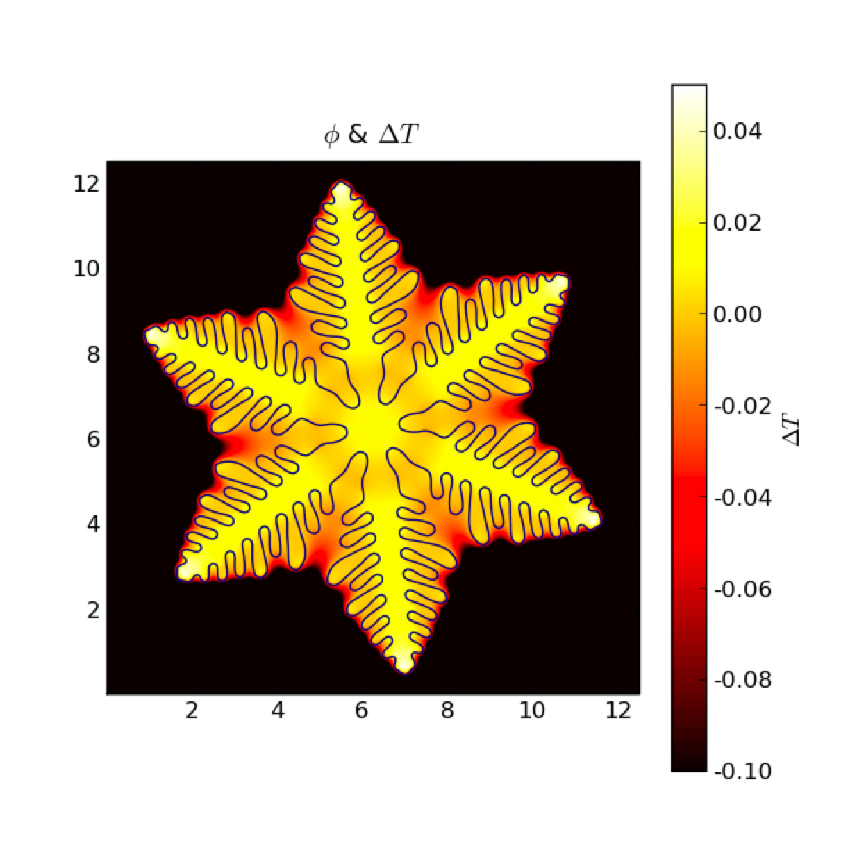
phase field and undercooling during solidification of a 6-fold "snowflake" anisotropic seed

The non-uniform temperature results from the release of latent heat at the solidifying interface. The dendrite arms grow fastest where the temperature gradient is steepest.

We note that this FiPy simulation is written in about 50 lines of code (excluding the custom viewer), compared with over 800 lines of (fairly lucid) FORTRAN code used for the figures in [13].

Last updated on Jun 27, 2023. Created using Sphinx 6.2.1.