FiPy
FiPy
![]()
Version 3.1
examples.cahnHilliard.mesh2D
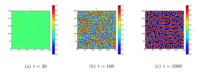
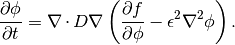
The spinodal decomposition phenomenon is a spontaneous separation of an initially homogenous mixture into two distinct regions of different properties (spin-up/spin-down, component A/component B). It is a “barrierless” phase separation process, such that under the right thermodynamic conditions, any fluctuation, no matter how small, will tend to grow. This is in contrast to nucleation, where a fluctuation must exceed some critical magnitude before it will survive and grow. Spinodal decomposition can be described by the “Cahn-Hilliard” equation (also known as “conserved Ginsberg-Landau” or “model B” of Hohenberg & Halperin)
where  is a conserved order parameter, possibly representing
alloy composition or spin.
The double-well free energy function
is a conserved order parameter, possibly representing
alloy composition or spin.
The double-well free energy function 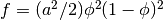 penalizes states with intermediate values of
between 0 and 1. The gradient energy term
penalizes states with intermediate values of
between 0 and 1. The gradient energy term  ,
on the other hand, penalizes sharp changes of .
These two competing effects result in the segregation
of into domains of 0 and 1, separated by abrupt, but
smooth, transitions. The parameters
,
on the other hand, penalizes sharp changes of .
These two competing effects result in the segregation
of into domains of 0 and 1, separated by abrupt, but
smooth, transitions. The parameters  and
and  determine the relative
weighting of the two effects and
determine the relative
weighting of the two effects and  is a rate constant.
We can simulate this process in FiPy with a simple script:
>>> from fipy import *
(Note that all of the functionality of NumPy is imported along with FiPy, although much is augmented for FiPy‘s needs.)
>>> if __name__ == "__main__":
...     nx = ny = 1000
... else:
...     nx = ny = 20
>>> mesh = Grid2D(nx=nx, ny=ny, dx=0.25, dy=0.25)
>>> phi = CellVariable(name=r"$\phi$", mesh=mesh)
We start the problem with random fluctuations about 
>>> phi.setValue(GaussianNoiseVariable(mesh=mesh,
...                                    mean=0.5,
...                                    variance=0.01))
FiPy doesn’t plot or output anything unless you tell it to:
>>> if __name__ == "__main__":
...     viewer = Viewer(vars=(phi,), datamin=0., datamax=1.)
For FiPy, we need to perform the partial derivative
 manually and then put the equation in the canonical
form by decomposing the spatial derivatives
so that each Term is of a single, even order:
manually and then put the equation in the canonical
form by decomposing the spatial derivatives
so that each Term is of a single, even order:
![\frac{\partial \phi}{\partial t}
= \nabla\cdot D a^2 \left[ 1 - 6 \phi \left(1 - \phi\right)\right] \nabla \phi- \nabla\cdot D \nabla \epsilon^2 \nabla^2 \phi.](../../../_images/math/b0b8bd746e18d11687942a235cf458940baec658.png)
FiPy would automatically interpolate D * a**2 * (1 - 6 * phi * (1 - phi)) onto the faces, where the diffusive flux is calculated, but we obtain somewhat more accurate results by performing a linear interpolation from phi at cell centers to PHI at face centers. Some problems benefit from non-linear interpolations, such as harmonic or geometric means, and FiPy makes it easy to obtain these, too.
>>> PHI = phi.arithmeticFaceValue
>>> D = a = epsilon = 1.
>>> eq = (TransientTerm()
...       == DiffusionTerm(coeff=D * a**2 * (1 - 6 * PHI * (1 - PHI)))
...       - DiffusionTerm(coeff=(D, epsilon**2)))
Because the evolution of a spinodal microstructure slows with time, we use exponentially increasing time steps to keep the simulation “interesting”. The FiPy user always has direct control over the evolution of their problem.
>>> dexp = -5
>>> elapsed = 0.
>>> if __name__ == "__main__":
...     duration = 1000.
... else:
...     duration = 1000.
>>> while elapsed < duration:
...     dt = min(100, numerix.exp(dexp))
...     elapsed += dt
...     dexp += 0.01
...     eq.solve(phi, dt=dt, solver=LinearLUSolver())
...     if __name__ == "__main__":
...         viewer.plot()
...     elif (max(phi.globalValue) > 0.7) and (min(phi.globalValue) < 0.3) and elapsed > 10.:
...         break
>>> print (max(phi.globalValue) > 0.7) and (min(phi.globalValue) < 0.3)
True