examples.cahnHilliard.sphere

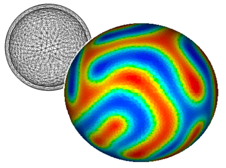
Solves the Cahn-Hilliard problem on the surface of a sphere.

This phenomenon can occur on vesicles (http://www.youtube.com/watch?v=kDsFP67_ZSE).

>>> from fipy import CellVariable, Gmsh2DIn3DSpace, GaussianNoiseVariable, Viewer, TransientTerm, DiffusionTerm, DefaultSolver
>>> from fipy.tools import numerix

The only difference from examples.cahnHilliard.mesh2D is the declaration of mesh.

>>> mesh = Gmsh2DIn3DSpace('''
...     radius = 5.0;
...     cellSize = 0.3;
...
...     // create inner 1/8 shell
...     Point(1) = {0, 0, 0, cellSize};
...     Point(2) = {-radius, 0, 0, cellSize};
...     Point(3) = {0, radius, 0, cellSize};
...     Point(4) = {0, 0, radius, cellSize};
...     Circle(1) = {2, 1, 3};
...     Circle(2) = {4, 1, 2};
...     Circle(3) = {4, 1, 3};
...     Line Loop(1) = {1, -3, 2} ;
...     Ruled Surface(1) = {1};
...
...     // create remaining 7/8 inner shells
...     t1[] = Rotate {{0,0,1},{0,0,0},Pi/2} {Duplicata{Surface{1};}};
...     t2[] = Rotate {{0,0,1},{0,0,0},Pi} {Duplicata{Surface{1};}};
...     t3[] = Rotate {{0,0,1},{0,0,0},Pi*3/2} {Duplicata{Surface{1};}};
...     t4[] = Rotate {{0,1,0},{0,0,0},-Pi/2} {Duplicata{Surface{1};}};
...     t5[] = Rotate {{0,0,1},{0,0,0},Pi/2} {Duplicata{Surface{t4[0]};}};
...     t6[] = Rotate {{0,0,1},{0,0,0},Pi} {Duplicata{Surface{t4[0]};}};
...     t7[] = Rotate {{0,0,1},{0,0,0},Pi*3/2} {Duplicata{Surface{t4[0]};}};
...
...     // create entire inner and outer shell
...     Surface Loop(100)={1,t1[0],t2[0],t3[0],t7[0],t4[0],t5[0],t6[0]};
... ''', overlap=2).extrude(extrudeFunc=lambda r: 1.1 * r) 
>>> phi = CellVariable(name=r"$\phi$", mesh=mesh) 

We start the problem with random fluctuations about

>>> phi.setValue(GaussianNoiseVariable(mesh=mesh,
...                                    mean=0.5,
...                                    variance=0.01)) 

FiPy doesn’t plot or output anything unless you tell it to: If MayaviClient is available, we can customize the view with a subclass of MayaviDaemon.

>>> if __name__ == "__main__":
...     try:
...         viewer = MayaviClient(vars=phi,
...                               datamin=0., datamax=1.,
...                               daemon_file="examples/cahnHilliard/sphereDaemon.py")
...     except:
...         viewer = Viewer(vars=phi,
...                         datamin=0., datamax=1.,
...                         xmin=-2.5, zmax=2.5)

For FiPy, we need to perform the partial derivative manually and then put the equation in the canonical form by decomposing the spatial derivatives so that each Term is of a single, even order:

FiPy would automatically interpolate D * a**2 * (1 - 6 * phi * (1 - phi)) onto the faces, where the diffusive flux is calculated, but we obtain somewhat more accurate results by performing a linear interpolation from phi at cell centers to PHI at face centers. Some problems benefit from non-linear interpolations, such as harmonic or geometric means, and FiPy makes it easy to obtain these, too.

>>> PHI = phi.arithmeticFaceValue 
>>> D = a = epsilon = 1.
>>> eq = (TransientTerm()
...       == DiffusionTerm(coeff=D * a**2 * (1 - 6 * PHI * (1 - PHI)))
...       - DiffusionTerm(coeff=(D, epsilon**2))) 

Because the evolution of a spinodal microstructure slows with time, we use exponentially increasing time steps to keep the simulation “interesting”. The FiPy user always has direct control over the evolution of their problem.

>>> dexp = -5
>>> elapsed = 0.
>>> if __name__ == "__main__":
...     duration = 1000.
... else:
...     duration = 1e-2
>>> while elapsed < duration:
...     dt = min(100, numerix.exp(dexp))
...     elapsed += dt
...     dexp += 0.01
...     eq.solve(phi, dt=dt, solver=DefaultSolver(precon=None)) 
...     if __name__ == "__main__":
...         viewer.plot()

Last updated on Jun 27, 2023. Created using Sphinx 6.2.1.