OOF2: The Manual
| Property | ||
|---|---|---|

|
8.6.3. Property- and Material-related Classes |  |
Name
Property — Base class for material properties
Synopses
C++ Synopsis
#include "engine/property.h"class Property {Property(const std::string& name,
PyObject* registration);virtual void cross_reference(Material* material);virtual void precompute();virtual void begin_element(const CSubProblem* subproblem,
const Element* element);virtual void begin_point(const FEMesh* mesh,
const Element* element,
const Flux* flux,
const MasterPosition& masterpos);virtual void end_point(const FEMesh* mesh,
const Element* element,
const Flux* flux,
const MasterPosition& masterpos);virtual void end_element(const CSubProblem* subproblem,
const Element* element);virtual void post_process(CSubProblem* mesh,
const Element* element) const;virtual int integration_order(const CSubProblem* mesh,
const Element* element) const;virtual void fluxmatrix(const FEMesh* mesh,
const Element* element,
const ElementFuncNodeIterator& node,
const Flux* flux,
const FluxData* fluxdata,
const MasterPosition& position) const;virtual void fluxrhs(const FEMesh* mesh,
const Element* element,
const Flux* flux,
FluxData* fluxdata,
MasterPosition& position) const;virtual void output(const FEMesh* mesh,
const Element* element,
const PropertyOutput* p_output,
const MasterPosition& position,
OutputVal* value) const;virtual bool is_symmetric(const CSubProblem* subproblem) const;
}
Python Synopsis
from oof2.SWIG.engine.pypropertywrapper import PyPropertyWrapperclass PyPropertyWrapper(Property):def __init__(self, referent, registration, name)def integration_order(self, subproblem, element)def cross_reference(self, material)def precompute(self)def begin_element(self, subproblem, element)def begin_point(self, mesh, element, flux, master_position)def end_point(self, mesh, element, flux, master_position)def end_element(self, subproblem, element)def post_process(self, subproblem, element)def fluxmatrix(self, mesh, element, node, flux, fluxdata, master_position)def fluxrhs(self, mesh, element, flux, fluxdata, master_position)def output(self, mesh, element, p_output, position)def is_symmetric(self, subproblem)
Overview
Property classes can be constructed either in C++ or Python.
Python classes are somewhat simpler to program and build, but
C++ classes are significantly more efficient, computationally.
In C++, new Properties are constructed by creating
subclasses of the Property class. In
Python, they're constructed by creating subclasses of the
PyPropertyWrapper class.
(PyPropertyWrapper is a swig wrapper
class around a C++ class of the same name, which is itself
derived from Property.) In both cases,
the base classes contain trivial implementations of all
methods except integration_order, so it
is safe to omit from the derived classes functions which are
irrelevant to a particular physical property. The
integration_order is always relevant to
the physical property to which it belongs.
In order for both C++ and Python Properties to work properly
and to be included in the GUI, every subclass must have an
associated PropertyRegistration
object. PropertyRegistrations must
always be created in Python, even for C++
Property subclasses.
Constructors
C++
C++ Property subclasses must have a
constructor of the form
SubProperty::SubProperty(PyObject *registration, const std::string& name, ...)
and they must invoke the base class constructor like this:[57]
Property(const std::string& name, PyObject *registration)
The derived class should treat name and
registration as opaque variables, used
only by the base class. They just need to be passed on
through. The ... in the subclass
constructor refers to the Property's
parameters, which must appear in the
constructor argument list in the same order that they appear
in the corresponding PropertyRegistration.
C++ Property classes should
not have a copy constructor. The base
class copy constructor is private, to prohibit unauthorized
duplication, by any means, electronic or otherwise.
Python
The Python constructor for a
PyPropertyWrapper subclass must look
like this:
def __init__(self, registration, name, ...):
    PyPropertyWrapper.__init__(self, registration, name)
As in the C++
constructor, the name and
registration parameters should be passed
through to the base class unchanged.
The ... in the constructor arguments
refers to any parameters that the
Property might have. These must have
the same names and be in the same order as the parameters in
the associated PropertyRegistration.
Methods
The following methods can be defined in C++
Property and Python
PyPropertyWrapper subclasses. Most are
optional, and can be omitted if the default behavior is
satisfactory. Unless otherwise noted, the default behavior is
to do nothing. The exception is
integration_order, which must be provided
explicitly for all properties. A base-class version does
exist, but its default behavior is to indicate an error.
All of the functions can be accessed from either C++ or Python. If there are non-obvious differences between the C++ and Python invocations, they are noted below. Minor and standard punctuation differences are not noted. Function prototypes are specified in the C++ format, because it is more informative.
void cross_reference(Material *)
cross_reference is called whenever
a new Property is added to a Material. It gives each
Property a chance to locate other Properties in the same
Material from which it may need information. For example,
many Properties of an anisotropic material will need to
know the Material's Orientation
Property. The argument to
cross_reference is the Material
object to which the Property belongs.
Material::fetchProperty
should be used to look for other
Properties. It will raise an
exception if the sought-for Property
does not exist. This exception should
not be caught by the
Property — it's handled in the
Material.
For example, here is the
cross_reference routine from the
AnisotropicThermalExpansion class,
which needs to access the Elasticity (for the elastic
modulus) and the Orientation:
void AnisotropicThermalExpansion::cross_reference(Material *mat) {
  elasticity = dynamic_cast<Elasticity*>(mat->fetchProperty("Elasticity"));
  orientation = dynamic_cast<OrientationProp*>(mat->fetchProperty("Orientation"));
}
The ThermalExpansion and
AnisotropicThermalExpansion classes
store the elasticity and
orientation variables:
class ThermalExpansion : public Property {
protected:
  Elasticity *elasticity;
  ...
};

class AnisotropicThermalExpansion : public ThermalExpansion {
private:
  OrientationProp *orientation;
  ...
};
The default base class
cross_reference function does
nothing.
void precompute()
precompute() is called when a Mesh is
being solved. It's called before any other
Property methods, other than
cross_reference. It should compute any
quantities that the Property needs
that depend only upon Property
data. It can use Property data from
other Properties, having located
those other Properties during the
cross_reference step.
For example, if a Property has an
anisotropic modulus, the Property's
precompute method should rotate the
modulus to lab coordinates using the Material's Orientation.
void begin_element(const CSubProblem*, const const Element*)
When building the finite element stiffness matrix and right
hand side vector, OOF2 loops over the elements of the mesh
and computes each element's contribution by calling each
Property's fluxmatrix
and fluxrhs
methods. Before calling these functions, however, it first
calls begin_element, passing the
current Element
as an argument. This allows the
Property to precompute any
Element dependent properties.
void end_element(const CSubProblem*, const Element*)
end_element is just like
begin_element,
except that it's called after OOF2 is
done computing an Element's
contribution. end_element can be
used to clean up any temporary objects allocated by
begin_element.
void begin_point(const FEMesh*, const const Element*, const Flux*, const MasterPosition&)
Within each element, OOF2 loops over gausspoints.
Property objects can use this
begin_point hook to perform expensive computations that are
required at an evaluation point, and cache the results.
There is a matching end_point
function which can be used to clear the cached data.
void end_point(const FEMesh*, const Element*, const Flux*, const MasterPosition&)
end_point is just like
begin_point,
except that it's called after OOF2 is
done computing the contribution at a point. The
end_point method can be used to
clean up any temporary objects allocated by
begin_point.
void post_process(CSubProblem*, const Element*)
After solving the finite element equations,
post_process is called once on each
Element in a
CSubProblem.
It can be used for any sort of post-processing, such as
adjusting material parameters, or generating output files.
Do not confuse post_process with
end_element.
end_element is called during finite
element matrix construction, before the equations are
solved.
int integration_order(const CSubProblem *subproblem, const Element
               	    *element) const
integration_order returns the polynomial
order (or degree) of the part of the flux matrix (computed
by fluxmatrix
or fluxrhs)
that this Property is responsible
for. All Properties that define
fluxmatrix
or fluxrhs
should define integration_order.
Because fluxmatrix and
fluxrhs use the finite element
shape functions and their derivatives,
integration_order must find out the
polynomial degree of the shapefunctions. The current mesh
Element is passed in as an argument.
The shapefunction's degree can be found by calling Element::shapefun_degree,
and it's derivative's degree can be found by calling Element::dshapefun_degree.
![[Warning]](IMAGES/warning.png) |
Warning |
|---|---|
|
Do not compute the shapefunction's
derivative's degree by subtracting 1 from the
shapefunction's degree. For purposes of Gaussian
integration, the degree of the shapefunction is sometimes
less than its actual polynomial degree. For example, the
linear quadrilateral shapefunction |
As an example, here is the
integration_order method for the
Elasticity class in OOF2. The
fluxmatrix routine always adds a
(constant) modulus times a shape function derivative to the
flux matrix, but when the displacement field has
out-of-plane components, there are terms proportional to the
shape functions as well.
integration_order must return the
largest relevant degree, so it has to check for out-of-plane
fields:
int Elasticity::integration_order(const CSubProblem *subproblem, const Element *el) const {
  if(displacement->in_plane(subproblem))
    return el->dshapefun_degree();
  return el->shapefun_degree();
}
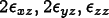
void fluxmatrix(...)
OOF2 Properties that represent
terms in a constitutive equation must define the function
Property::fluxmatrix.
fluxmatrix computes a matrix that,
when multiplied by a vector of degrees of freedom, produces
a vector containing the components of a Flux. Explaining
this properly requires a brief review of the finite element
machinery.
Let  be the nth
component of a field
be the nth
component of a field  at position
 .
If the field values are known at nodes
.
If the field values are known at nodes  at positions
 , then the finite element shape functions
 can be used to approximate the field at any point:
![\[u_n({\bf r}) = \sum_\nu
N_\nu({\bf r}) u_{n\nu}\]](equations/8.6.3-eq-1.gif)
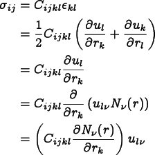
where
 is the shape function that is 1 at node
 and 0 at all other nodes, and
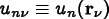 .
.
A constitutive relation connects a Field,  , and a
Flux,  , through a modulus. For now, let's assume
that it can be represented as a linear operator,
, through a modulus. For now, let's assume
that it can be represented as a linear operator,
 :
:
![\[\sigma({\bf r}) = M({\bf r})\cdot u({\bf r})\]](equations/8.6.3-eq-2.gif)
Inserting (8.2) into
(8.3) shows that
 can be written as a matrix, which we call the flux
matrix. The columns of
can be written as a matrix, which we call the flux
matrix. The columns of  correspond to
degrees of freedom
correspond to
degrees of freedom  , and its rows to
components of the flux
, and its rows to
components of the flux
 .
.
For example, for elasticity
from which we get
![\[
M_{ij,l\nu} = C_{ijkl}\frac{\partial N_\nu(r)}{\partial r_k}
\]](equations/8.6.3-eq-4.gif)
Repeated indices are summed in all of the above equations. In particular, in (8.5), k runs only over the in-plane components x and y.
Actually, (8.5) isn't quite
correct, because we ignored the out-of-plane
components. The out-of-plane part of the displacement field
is the vector of derivatives
 , which is just
 (using the fact that
  and
and  must both be zero).
The part of the flux
must both be zero).
The part of the flux  due to the out-of-plane strains is
![\[
\sigma_{ij} =
\frac12\left[C_{ijxz}\frac{\partial u_z}{\partial x}
+C_{ijyz}\frac{\partial u_z}{\partial y}\right]
+ C_{ijzz}\frac{\partial u_z}{\partial z}
\]](equations/8.6.3-eq-5.gif)
Since  is the
 component of a field (an out-of-plane field, in the OOF2
sense — it's computed at nodes just like in-plane
fields are), it can be expanded in terms of shape functions
and the field values at nodes, as in (8.2). From this we see that
the extra terms in
component of a field (an out-of-plane field, in the OOF2
sense — it's computed at nodes just like in-plane
fields are), it can be expanded in terms of shape functions
and the field values at nodes, as in (8.2). From this we see that
the extra terms in  are:
are:
![\[
M'_{ij,k\nu} = \frac12 C_{ijzk}(1+\delta_{kz})N_\nu
\]](equations/8.6.3-eq-6.gif)
(Note:
 is not
summed in (8.7).)
is not
summed in (8.7).)
On each call, fluxmatrix must make
contributions to  for all of the
components of a given flux (
for all of the
components of a given flux ( ), all of the
components of the relevant fields (
), all of the
components of the relevant fields ( and its out-of-plane part), and one given node
(
and its out-of-plane part), and one given node
( ).
).
It is important to note that it is not
necessary for the fluxmatrix
routine or its author to know anything about the following:
-
The topology or number of nodes in the element.
-
How nodal degrees of freedom are mapped into columns of the flux matrix.
-
How flux components are mapped into rows of the flux matrix.
-
What equations are being solved.
The arguments to fluxmatrix are:
const FEMesh *mesh-
The finite element mesh that's being solved.
fluxmatrixprobably doesn't have to use themeshobject directly, but it does have to pass it through to other functions. const Element *element-
The finite element under consideration. This shouldn't be explicitly needed except in cases in which the material parameters depend on physical space coordinates or in which history-dependent fields are stored in the element.
const ElementFuncNodeIterator &node-
This is the node
 referred to in the discussion above. Its
passed in in the guise of an iterator, which can
iterate over all of the nodes of the element,
although it should be thought of here simply as a
way of accessing the node's indices and shape
functions.[58]
The node's shape function and its
derivatives can be obtained from
referred to in the discussion above. Its
passed in in the guise of an iterator, which can
iterate over all of the nodes of the element,
although it should be thought of here simply as a
way of accessing the node's indices and shape
functions.[58]
The node's shape function and its
derivatives can be obtained from ElementFuncNodeIterator::shapefunctionandElementFuncNodeIterator::dshapefunction. const Flux *flux-
The
Flux referred to in the discussion above.
Properties that contribute to more than one
referred to in the discussion above.
Properties that contribute to more than one Fluxneed to check this variable to know which flux they're computing now. FluxData *fluxdata-
The
FluxDataclass stores the actual flux matrix and other
flux data. (This data can't be stored directly in
the
and other
flux data. (This data can't be stored directly in
the Fluxobject because oneFluxis shared among manyFEMeshes. TheFluxDataobject is local to this computation.) The actual flux matrix can be accessed
only through the method
can be accessed
only through the method FluxData::matrix_element. This function handles the mapping from node, field, and flux component indices to actual row and column indices. const MasterPosition &x-
The flux matrix is evaluated at a physical coordinate
 (often a Gauss integration point, but not always).
xis the point in theElement's master coordinate space[59] corresponding to r.
Here is the fluxmatrix routine for
the Elasticity class, from
SRC/engine/property/elasticity/elasticity.C
in the OOF2 source code:
void Elasticity::fluxmatrix(const FEMesh *mesh, const Element *element,
const ElementFuncNodeIterator &nu,
const Flux *flux, FluxData *fluxdata,
const MasterPosition &x) const
{
if(*flux != *stress_flux) {  throw ErrProgrammingError("Unexpected flux", __FILE__, __LINE__);
  }
const Cijkl modulus = cijkl(mesh, element, x);
}
const Cijkl modulus = cijkl(mesh, element, x);  double sf = nu.shapefunction(x);
  double dsf0 = nu.dshapefunction(0, x);
  double dsf1 = nu.dshapefunction(1, x);
for(SymTensorIterator ij; !ij.end(); ++ij) {
double dsf1 = nu.dshapefunction(1, x);
for(SymTensorIterator ij; !ij.end(); ++ij) {  for(IteratorP ell=displacement->iterator(); !ell.end(); ++ell) {
  SymTensorIndex ell0(0, ell.integer());
  SymTensorIndex ell1(1, ell.integer());
fluxdata->matrix_element(mesh, ij, displacement, ell, nu) +=
SymTensorIndex ell1(1, ell.integer());
fluxdata->matrix_element(mesh, ij, displacement, ell, nu) +=  modulus(ij, ell0)*dsf0 + modulus(ij, ell1)*dsf1;
  }
if(!displacement->in_plane(mesh)) {
}
if(!displacement->in_plane(mesh)) {  Field *oop = displacement->out_of_plane();
  for(IteratorP ell=oop->iterator(ALL_INDICES); !ell.end(); ++ell) {
  double diag_factor = ( ell.integer()==2 ? 1.0 : 0.5);
  fluxdata->matrix_element(mesh, ij, oop, ell, nu) +=
  modulus(ij, SymTensorIndex(2, ell.integer())) * sf * diag_factor;
  }
}
}
}
}
}
}
} |
|
We don't really need to do this. It's a sanity check to
make sure that we got the |
|
|
|
|
|
|
|
|
Here is where the shape functions are evaluated. This
is |
|
|
These are the derivatives of the shape functions. The
first argument is the component of the
gradient. |
|
|
This is the loop over components of the flux. We know
that the flux (stress) is a symmetric tensor, so we use
a for(IteratorP ij = flux->iterator(); !ij.end(); ++ij) ... The loop here extends over all components of the stress, without regard to whether or not the stress is in-plane. That's because the out-of-plane components of the flux matrix are used to construct the plane-stress constraint equation. |
|
|
This is the loop over the in-plane
components of the displacement field. In this case it's
been written in the generic form.
|
|
|
This simply creates a
|
|
|
This retrieves a C++ reference to the matrix element
that couples flux component |
|
|
The two terms in this line are the implied sum over
|
|
|
If the displacement field has no out-of-plane part, we don't need to compute the out-of-plane part's contributions to the stress. |
|
|
This retrieves the |
|
|
This loops over the components of the out-of-plane
field. Since this field has three components
( |
|
|
This takes care of the numerical factor in (8.7). All |
|
|
This line is just like |
|
|
This is the right hand side of (8.7). |


void Property::fluxrhs(...) const
OOF2 Properties that represent
external (generalized) forces or otherwise contribute to the
right hand side of a divergence
equation must define
Property::fluxrhs.
fluxrhs is similar to Property::fluxmatrix
in its role and its arguments, but is generally simpler to
implement. Each fluxrhs
implementation must compute a quantity at a given point
within an element, but does not have to concern itself with
nodes and shapefunctions.
There are two kinds of contributions to the right hand side
of the divergence equation. Body
forces contribute directly to the right hand side
of the divergence equation (2.8),
but offsets contribute a
field-independent value to the flux on the left hand side of
(2.8).
(Field-dependent contributions are made
by Property::fluxmatrix.)
For an example, consider linear thermal expansion. The flux (stress) is
![\[
\sigma_{ij} = C_{ijkl}
\left(\epsilon_{kl} - \alpha_{kl}(T-T_0)\right)
\]](equations/8.6.3-eq-7.gif)
 is the temperature at which the stress-free strain vanishes,
and makes a field independent offset,
is the temperature at which the stress-free strain vanishes,
and makes a field independent offset,
 ,
to the flux. On the other hand, gravitational forces do not
contribute to the flux, but appear as body forces:
,
to the flux. On the other hand, gravitational forces do not
contribute to the flux, but appear as body forces:
![\[\nabla\cdot\sigma = -g\hat{\mathrm{\bf y}}\]](equations/8.6.3-eq-8.gif)
The arguments to Property::fluxrhs are:
const FEMesh *mesh-
The finite element mesh that's being solved.
fluxrhsprobably doesn't have to use themeshobject directly, but it might need to pass it through to other functions. const Element *element-
The finite element under consideration. This shouldn't be explicitly needed except in cases in which the material parameters depend on physical space coordinates or in which history-dependent fields are stored in the element.
const Flux *flux-
The
Fluxunder consideration. FluxData *fluxdata-
The
fluxdataobject stores the results computed byfluxrhs. It's the same object that was passed tofluxmatrix.FluxData::offset_elementaccumulates offsets, andFluxData::rhs_elementaccumulates body forces. const MasterPosition &x-
Each call to
fluxrhsevaluates the rhs or flux offset at a given point within the givenElement.xis the master space[59] coordinate of the point.
Here is the fluxrhs function from
the ForceDensity class, from
SRC/engine/property/forcedensity/forcedensity.C
in the OOF2 source code. It provides an example of a
body force:
void ForceDensity::fluxrhs(const FEMesh *mesh, const Element *element,
const Flux *flux, FluxData *fluxdata,
const MasterPosition &x) const
{
if(*flux != *stress_flux) {
throw ErrProgrammingError("Unexpected flux", __FILE__, __LINE__);
}
fluxdata->rhs_element(0) -= gx;
fluxdata->rhs_element(1) -= gy;
} |
|
As in |
|||
|
|
|
|||
|
|
|
![[Note]](IMAGES/note.png)
Here is the fluxrhs method from the
ThermalExpansion property, which is
an example of a flux offset. It
computes the field-independent term

The original version can be found in
SRC/engine/property/thermalexpansion/thermalexpansion.C
in the OOF2 source code.
void ThermalExpansion::fluxrhs(const FEMesh *mesh, const Element *element,
				   const Flux *flux, FluxData *fluxdata,
				   const MasterPosition &x) const {

  if(*flux!=*stress_flux) {
    throw ErrProgrammingError("Unexpected flux." __FILE__, __LINE__);
  }
  const Cijkl modulus = elasticity->cijkl(mesh, element, x);

  for(SymTensorIterator ij; !ij.end(); ++ij) {
    double &offset_el = fluxdata->offset_element(mesh, ij);
    for(SymTensorIterator kl; !kl.end(); ++kl) {
      if(kl.diagonal()) {
	offset_el += modulus(ij,kl)*expansiontensor[kl]*tzero_;
      }
      else {
	offset_el += 2.0*modulus(ij,kl)*expansiontensor[kl]*tzero_;
      }
    }
  }
} |
|
This retrieves the elastic modulus
void ThermalExpansion::cross_reference(Material *mat) {
  elasticity = dynamic_cast<Elasticity*>(mat->fetchProperty("Elasticity"));
}
|
|
|
This is the loop over components of the flux, just like
item |
|
|
|
|
|
This is the loop over the indices
|
|
|
The next few lines compute terms in the sum,
accumulating them in the |


void output(..)
A Property's
output function is called when
quantities that depend on the
Property are being computed, usually
(but not necessarily) after a solution has been obtained on
a mesh. Many different kinds of
PropertyOutputs can be defined (see
Section 8.5). Each
Property class's PropertyRegistration
indicates which kinds of
PropertyOutput the
Property can compute. The
output function must determine
which PropertyOutput is being
computed, get the output's parameter values if necessary,
compute its value at a given point in the mesh, and store
the value in a given OutputVal
object.
The arguments to Property::output
in C++ are:
const FEMesh *mesh-
The mesh on which the output is being computed. The
outputfunction will probably not need to use this variable directly, but must pass it through to other functions. const Element *element-
The element of the mesh containing the point at which output values are desired.
const PropertyOutput *output-
The
PropertyOutputobject being computed. The object is created by the OOF2 menu system and, depending on the type of output, may contain Python arguments specifying exactly what's to be computed. For example, a strain output will specify whether it's computing the total, elastic, thermal or other variety of strain. See the example below. const MasterPosition & pos-
The position in the element's master coordinate space[59] at which the output is to be computed.
OutputVal *data-
The object in which the computed data should be stored. In C++, the object must be first cast to an appropriate derived type. The new value should be added to
data, to ensure that values computed by otherPropertiesare retained.
In Python, the arguments are the same, except that there's
no data argument. Instead, the function
returns an OutputVal
(of the appropriate type) containing the
Property's contribution to the output
quantity.
Here is an example of a fairly complicated
output function, from
SRC/engine/property/thermalexpansion/thermalexpansion.C
in the OOF2 source code. It computes one of two types of
output, Strain and
Energy, each of which has two variants.
void ThermalExpansion::output(const FEMesh *mesh,
				  const Element *element,
				  const PropertyOutput *output,
				  const MasterPosition &pos,
				  OutputVal *data)
  const
{
  const std::string &outputname = output->name();
  if(outputname == "Strain") {
    // The parameter is a Python StrainType instance.  Extract its name.
    std::string stype = output->getRegisteredParamName("type");
    SymmMatrix3 *sdata = dynamic_cast<SymmMatrix3*>(data);
    // Compute alpha*T with T interpolated to position pos
    const OutputValue tfield = element->outputField(mesh, *temperature, pos);
    const ScalarOutputVal *tval =
      dynamic_cast<const ScalarOutputVal*>(tfield.valuePtr());
    double t = tval->value();

    if(stype == "Thermal")
      *sdata += expansiontensor*(t-tzero_);
    else if(stype == "Elastic")
      *sdata -= expansiontensor*(t-tzero_);
  } // strain output ends here

  if(outputname == "Energy") {
    // The parameter is a Python Enum instance.  Extract its name.
    std::string etype = output->getEnumParam("etype");
    if(etype == "Total" || etype == "Elastic") {
      ScalarOutputVal *edata =
	dynamic_cast<ScalarOutputVal*>(data);
      SymmMatrix3 thermalstrain;
      const Cijkl modulus = elasticity->cijkl(mesh, element, pos);
      const OutputValue tfield = element->outputField(mesh, *temperature, pos);
      const ScalarOutputVal *tval =
	dynamic_cast<const ScalarOutputVal*>(tfield.valuePtr());
      double t = tval->value();
      thermalstrain = expansiontensor*(t-tzero_);
      SymmMatrix3 thermalstress(modulus*thermalstrain);
      SymmMatrix3 strain;
      findGeometricStrain(mesh, element, pos, strain);
      double e = 0;
      for(int i=0; i<3; i++) {
	e += thermalstress(i,i)*strain(i,i);
	int j = (i+1)%3;
	e += 2*thermalstress(i,j)*strain(i,j);
      }
      *edata += -0.5*e;
    }
  } //energy output ends here
} |
|
The name of the output indicates what type of quantity is to be computed. |
|
|
This call to
|
|
|
Because we know that this is a |
|
|
temperature = dynamic_cast<ScalarField*>(Field::getField("Temperature"));
This line calls |
|
|
This line peels off the wrapper around the |
|
|
This line extracts the actual temperature from the
|
|
|
These lines add the thermal expansion contribution to
the strain, with the appropriate sign (depending on the
type of strain being computed).
|
|
|
The |
|
|
There are many different types of
|
|
|
Energy is a scalar, so the
|
|
|
See |
|
|
See |
|
|
|
|
|
This loop computes the contribution of thermal expansion to the elastic energy. |


bool is_symmetric(const CSubProblem *mesh) const
is_symmetric indicates whether or
not the finite element stiffness matrix constructed from the
Property can be made symmetric by
using the relationships
established by ConjugatePair
calls.
In most cases is_symmetric will simply
return true, if the matrix can be
symmetrized, or false, if it can't. Some
cases are more complicated, however. For example, thermal
expansion makes the matrix asymmetric if the temperature
field is an active field, because the thermal expansion
Property couples the temperature
(with no derivatives) to the gradient
of the displacement. Therefore, in the
ThermalExpansion class,
is_symmetric is defined like this:
bool ThermalExpansion::is_symmetric(const CSubProblem* subproblem) const {
  Equation *forcebalance = Equation::getEquation("Force_Balance");
  return !(forcebalance->is_active(subproblem) &&
	   temperature->is_defined(subproblem) &&
	   temperature->is_active(subproblem));
} [57] Sorry about the inconsistent order of the arguments.
[58]
It's not possible to use a Node
instead of an ElementFuncNodeIterator
here. Nodes are unable
to evaluate shape functions because they don't
know which Element
is being computed.
ElementFuncNodeIterators
know which Element
they're looping over.
[59]
Elements are first defined in a master
coordinate space, where geometry is easy, and
then mapped to their actual positions in
physical space. The master quadrilateral is a
square of side 2 centered on the origin. The
master triangle is a right isosceles triangle
with vertices (0,0), (1,0), and (0,1). A master
space coordinate can be converted to a physical
point by Element::from_master.
[60]
If the flux is in-plane, then
 and the out-of-plane force must be zero too. If
the flux is not in-plane, then
and the out-of-plane force must be zero too. If
the flux is not in-plane, then
 will be found during the solution process, and
the out-of-plane forces can be computed. In
both cases it's meaningless to specify the
forces ahead of time.
will be found during the solution process, and
the out-of-plane forces can be computed. In
both cases it's meaningless to specify the
forces ahead of time.
[61] This method of obtaining a field value may seem baroque, especially for a scalar field, but it's necessary for preserving generality. We may implement a short-cut for scalar fields in the future.
|
|
 |
|
| Planarity |  |
PropertyRegistration |