relax_liquid - Methodology and code
Python imports
[1]:
# Standard library imports
from pathlib import Path
import shutil
import datetime
from copy import deepcopy
from math import floor
from typing import Optional, Tuple
import random

# http://www.numpy.org/
import numpy as np

# https://ipython.org/
from IPython.display import display, Markdown

import matplotlib.pyplot as plt

# https://github.com/usnistgov/atomman
import atomman as am
import atomman.lammps as lmp
import atomman.unitconvert as uc
from atomman.tools import filltemplate

# https://github.com/usnistgov/iprPy
import iprPy
from iprPy.tools import read_calc_file

print('Notebook last executed on', datetime.date.today(), 'using iprPy version', iprPy.__version__)
Notebook last executed on 2022-10-17 using iprPy version 0.11.4
1. Load calculation and view description
1.1. Load the calculation
[2]:
# Load the calculation being demoed
calculation = iprPy.load_calculation('relax_liquid')
1.2. Display calculation description and theory
[3]:
# Display main docs and theory
display(Markdown(calculation.maindoc))
display(Markdown(calculation.theorydoc))
relax_liquid calculation style
Lucas M. Hale, lucas.hale@nist.gov, Materials Science and Engineering Division, NIST.
Introduction
The relax_liquid calculation style is designed to generate and characterize a liquid phase configuration for an atomic potential based on an initial configuration, target temperature and target pressure. The calculation involves multiple stages of relaxation and computes the mean squared displacement and radial distribution functions on the final liquid.
Version notes
2022-10-??: Calculation created
Additional dependencies
Disclaimers
No active checks are performed by this calculation to ensure that the system is liquid. Be sure to check the final atomic configurations. The thermo output can also provide a rough guideline in that you should see convergence of volume but not of the individual lx, ly, lz dimensions for a liquid phase.
If starting with a crystalline configuration, be sure to use an adequately high melt temperature and number of melt steps.
The temperature and volume equilibrium stages are designed to get the final nve system close to the target temperature and pressure, but they will not be exact. Be sure to check that the measured temperature and pressure are close to the targets.
Method and Theory
This performs five stages of simulations to create and analyze a liquid phase at a given temperature and pressure.
A “melt” stage is performed using npt at the target pressure and an elevated melt temperature.
A “cooling” stage is performed using npt in which the temperature is linearly reduced from the melt to the target temperature.
A “volume equilibrium” stage is performed using npt at the target temperature and pressure. Following the run, the system’s dimensions are equally scaled to the average volume.
A “temperature equilibrium” stage is performed using nvt at the target temperature. Following the run, the atomic velocities are scaled based on the expected total energy at the target temperature.
An “nve analysis” stage is performed in which the mean squared displacements of the atoms and the radial distribution function are measured.
Melt stage
The melt stage subjects the initial configuration to an npt simulation at the elevated melt temperature. This stage is meant to transform initially crystalline system configurations into amorphous liquid phases. As such, the melt temperature should be much higher than the melting temperature of the initial crystal, and the number of MD steps during this stage should be sufficiently high to allow for the phase transformation to occur.
If the initial atomic configuration is already amorphous, this stage can be skipped by setting meltsteps = 0. Also, if the initial configuration already has velocities assigned to the atoms, you can use those velocities by setting createvelocities = False. These two options make it possible to run a single melt simulation that can be used as the basis for all target temperatures. Note that createvelocities = True is needed if you want to measure statistical error from multiple runs.
Cooling stage
The cooling stage runs npt and linearly scales the temperature from the melt temperature to the target temperature. The larger the number of coolsteps, the more gradual the change from melt to target temperatures will be. This can be important if the target temperature is much smaller than the melt temperature.
Similarly to the melt stage, this stage can be skipped by setting coolsteps = 0. If meltsteps = coolsteps = 0 and createvelocities = True, the atomic velocities will be created for the system at the target temperature rather than the melt temperature. This allows for a generic amorphous state to be used as the starting configuration.
Volume equilibration stage
The volume equilibration stage runs npt at the target temperature and pressure. It is meant to allow for the system to equilibrate at the target temperature, then to obtain a time-averaged measurement of the system’s volume. The average volume is computed from a specified number of samples (volrelaxsamples) taken every 100 timesteps from the end of this stage. The max value allowed for volrelaxsamples is volrelaxsteps / 100, but practically it should be noticeably smaller than this to ignore measurements at the beginning of the stage where the system has not yet equilibrated.
When this stage finishes, the volume of the configuration cell is adjusted to the average volume computed by scaling each box length and tilt by the same factor, s
Temperature equilibration stage
The temperature equilibration stage runs nvt at the target temperature for the system fixed at the computed average volume. This allows for the system to equilibrate at the fixed volume and target temperature, and to compute a target total energy, \(E_{target}\), that corresponds to the system in equilibrium at the target temperature. \(E_{target}\) is computed based on time-averaged energy values from a specified number of samples (temprelaxsamples) taken every 100 timesteps from the end of this stage. The max value allowed for temprelaxsamples is temprelaxsteps / 100. Unlike the previous stage, the equilibration portion of this stage is likely negligible, therefore it is less important to ignore the initial measurements.
In LAMMPS, the adjustment is made by scaling all atomic velocities to a temperature \(T_s\) such that the current potential energy, \(E_{pot}\), plus the kinetic energy for \(T_s\) equals \(E_{target}\)
Two alternate methods for computing \(E_{target}\) are implemented and can be accessed with the temprelaxstyle option.
For temprelaxstyle = ‘te’, the target total energy is taken as the computed mean total energy
For temprelaxstyle = ‘pe’, the target total energy is taken as the computed mean potential energy plus kinetic energy for the target temperature, \(T\)
Limited tests show the two methods to result in mean temperatures in the final stage that have roughly the same variation from the target temperature, with ‘pe’ style giving slightly better results. As such, both methods are included as options and ‘pe’ is set as the default.
Analysis stage
The analysis stage runs nve with the system that has been adjusted to the target volume and total energy from the last two stages. During this stage, mean squared displacements and radial distribution function calculations are performed that can be used to analyze the liquid phase at the target temperature and pressure.
In addition to the analysis calculations, the average measured temperature and pressure are reported, which can be used as verification that the volume and temperature equilibration stages and adjustments worked properly.
2. Define calculation functions and generate files
This section defines the calculation functions and associated resource files exactly as they exist inside the iprPy package. This allows for the code used to be directly visible and modifiable by anyone looking to see how it works.
2.1. relax_liquid()
This is the primary function for the calculation. The version of this function built in iprPy can be accessed by calling the calc() method of an object of the associated calculation class.
[4]:
def relax_liquid(lammps_command: str,
                 system: am.System,
                 potential: lmp.Potential,
                 temperature: float,
                 mpi_command: Optional[str] = None,
                 pressure: float = 0.0,
                 temperature_melt: float = 3000.0,
                 meltsteps: int = 50000,
                 coolsteps: int = 10000,
                 volrelaxsteps: int = 50000,
                 volrelaxsamples: int = 300,
                 temprelaxsteps: int = 10000,
                 temprelaxsamples: int = 100,
                 temprelaxstyle: str = 'pe',
                 runsteps: int = 50000,
                 dumpsteps: Optional[int] = None,
                 createvelocities: bool = True,
                 randomseed: Optional[int] = None) -> dict:
    """
    Performs a multi-stage simulation to obtain a liquid phase configuration
    at a given temperature. Radial displacement functions and mean squared
    displacements are automatically computed for the system.

    Parameters
    ----------
    lammps_command :str
        Command for running LAMMPS.
    system : atomman.System
        The system to perform the calculation on.
    potential : atomman.lammps.Potential
        The LAMMPS implemented potential to use.
    temperature : float
        The target temperature to relax to.
    mpi_command : str, optional
        The MPI command for running LAMMPS in parallel.  If not given, LAMMPS
        will run serially.
    pressure : float, optional
        The target hydrostatic pressure to relax to. Default value is 0. GPa.
    temperature_melt : float, optional
        The elevated temperature to first use to hopefully melt the initial
        configuration.
    meltsteps : int, optional
        The number of npt integration steps to perform at the melt temperature
        to create an amorphous liquid structure.  Default value is 50000.
    coolsteps : int, optional
        The number of npt integration steps to perform to reduce the
        temperature from the melt temperature to the target temperature.
        Default value is 10000.
    volrelaxsteps : int, optional
        The number of npt integration steps to perform on the amorphous
        structure at the target temperature and pressure to obtain the
        equilibrium volume.  Default value is 50000.
    volrelaxsamples : int, optional
        The number of thermo samples from the end of the volume relax stage
        to use in computing the average volume.  Cannot be larger than
        volrelaxsteps / 100.  It is recommended to set smaller than the max
        to allow for some convergence time.  Default value is 300.
    temprelaxsteps : int, optional
        The number of nvt integration steps to perform on the system at
        the target temperature after scaling to the average equilibrium
        volume.  Default value is 10000.
    temprelaxsamples : int, optional
        The number of thermo samples from the end of the temperature relax
        stage to use in computing the target total energy.  Cannot be
        larger than temprelaxsteps / 100.  Default value is 100.
    temprelaxstyle : str, optional
        Indicates which scheme to use for computing the target total energy.
        Allowed values are 'pe' or 'te'.  For 'te', the average total energy
        from the temprelaxsamples is used as the target energy.  For 'pe',
        the average potential energy plus 3/2 N kB T is used as the target
        energy.  Default value is 'pe'.
    runsteps : int or None, optional
        The number of nve integration steps to perform on the system to
        obtain measurements of MSD and RDF of the liquid. Default value is
        50000.
    dumpsteps : int or None, optional
        Dump files will be saved every this many steps during the runsteps
        simulation. Default is None, which sets dumpsteps equal to runsteps.
    createvelocities : bool, optional
        If True (default), velocities will be created for the atoms prior to
        running the simulations.  Setting this to False can be useful if the
        initial system already has velocity information.
    randomseed : int or None, optional
        Random number seed used by LAMMPS in creating velocities and with
        the Langevin thermostat.  Default is None which will select a
        random int between 1 and 900000000.

    Returns
    -------
    dict
        Dictionary of results consisting of keys:

        - **'dumpfile_final'** (*str*) - The name of the final dump file
          created.
        - **'symbols_final'** (*list*) - The symbols associated with the final
          dump file.
        - **'volume'** (*float*) - The volume per atom identified after the volume
          equilibration stage.
        - **'volume_stderr'** (*float*) - The standard error in the volume per atom
          measured during the volume equilibration stage.
        - **'E_total'** (*float*) - The total energy of the system used during the nve
          stage.
        - **'E_total_stderr'** (*float*) - The standard error in the mean total energy
          computed during the energy equilibration stage.
        - **'E_pot'** (*float*) - The mean measured potential energy during the energy
          equilibration stage.
        - **'E_pot_stderr'** (*float*) - The standard error in the mean potential energy
          during the energy equilibration stage.
        - **'measured_temp'** (*float*) - The mean measured temperature during the nve
          stage.
        - **'measured_temp_stderr'** (*float*) - The standard error in the measured
          temperature values of the nve stage.
        - **'measured_press'** (*float*) - The mean measured pressure during the nve
          stage.
        - **'measured_press_stderr'** (*float*) - The standard error in the measured
          pressure values of the nve stage.
        - **'time_values'** (*numpy.array of float*) - The values of time that
          correspond to the mean squared displacement values.
        - **'msd_x_values'** (*numpy.array of float*) - The mean squared displacement
          values only in the x direction.
        - **'msd_y_values'** (*numpy.array of float*) - The mean squared displacement
         values only in the y direction.
        - **'msd_z_values'** (*numpy.array of float*) - The mean squared displacement
         values only in the z direction.
        - **'msd_values'** (*numpy.array of float*) - The total mean squared
           displacement values.
        - **'lammps_output'** (*atomman.lammps.Log*) - The LAMMPS logfile output.
          Can be useful for checking the thermo data at each simulation stage.
    """

    if temprelaxstyle not in ['pe', 'te']:
        raise ValueError('invalid temprelaxstyle option: must be "pe" or "te"')

    # Get lammps units
    lammps_units = lmp.style.unit(potential.units)

    #Get lammps version date
    lammps_date = lmp.checkversion(lammps_command)['date']

    # Handle default values
    if dumpsteps is None:
        dumpsteps = runsteps

    # Check volrelax and temprelax settings
    if volrelaxsamples > volrelaxsteps / 100:
        raise ValueError('invalid values: volrelaxsamples must be <= volrelaxsteps / 100')
    if temprelaxsamples > temprelaxsteps / 100:
        raise ValueError('invalid values: temprelaxsamples must be <= temprelaxsteps / 100')

    # Define lammps variables
    lammps_variables = {}

    lammps_variables['boltzmann'] = uc.get_in_units(uc.unit['kB'],
                                                    lammps_units['energy'])

    # Dump initial system as data and build LAMMPS inputs
    system_info = system.dump('atom_data', f='init.dat',
                              potential=potential)
    lammps_variables['atomman_system_pair_info'] = system_info

    # Phase settings
    lammps_variables['temperature'] = temperature
    lammps_variables['temperature_melt'] = temperature_melt
    lammps_variables['pressure'] = pressure

    # Set timestep dependent parameters
    timestep = lmp.style.timestep(potential.units)
    lammps_variables['timestep'] = timestep
    lammps_variables['temperature_damp'] = 100 * timestep
    lammps_variables['pressure_damp'] = 1000 * timestep

    # Number of run/dump steps
    lammps_variables['meltsteps'] = meltsteps
    lammps_variables['coolsteps'] = coolsteps
    lammps_variables['volrelaxsteps'] = volrelaxsteps
    lammps_variables['temprelaxsteps'] = temprelaxsteps
    lammps_variables['runsteps'] = runsteps
    lammps_variables['dumpsteps'] = dumpsteps

    # Number of samples
    lammps_variables['volrelaxsamples'] = volrelaxsamples
    lammps_variables['temprelaxsamples'] = temprelaxsamples

    # Set randomseed
    if randomseed is None:
        randomseed = random.randint(1, 900000000)
    #lammps_variables['randomseed'] = randomseed

    # create velocities
    if createvelocities:
        if meltsteps == 0 and coolsteps == 0:
            velocity_temp = temperature
        else:
            velocity_temp = temperature_melt
        lammps_variables['create_velocities'] = f'velocity all create {velocity_temp} {randomseed} mom yes rot yes dist gaussian'
    else:
        lammps_variables['create_velocities'] = ''

    # Set dump_keys based on atom_style
    if potential.atom_style in ['charge']:
        lammps_variables['dump_keys'] = 'id type q xu yu zu c_pe vx vy vz'
    else:
        lammps_variables['dump_keys'] = 'id type xu yu zu c_pe vx vy vz'

    # Set dump_modify_format based on lammps_date
    if lammps_date < datetime.date(2016, 8, 3):
        if potential.atom_style in ['charge']:
            lammps_variables['dump_modify_format'] = f'"%d %d{8 * " %.13e"}"'
        else:
            lammps_variables['dump_modify_format'] = f'"%d %d{7 * " %.13e"}"'
    else:
        lammps_variables['dump_modify_format'] = 'float %.13e'

    # Write lammps input script
    lammps_script = 'liquid.in'
    lammps_template = f'liquid_ave_{temprelaxstyle}.template'
    template = read_calc_file('iprPy.calculation.relax_liquid', lammps_template)
    with open(lammps_script, 'w') as f:
        f.write(filltemplate(template, lammps_variables, '<', '>'))

    # Run lammps
    output = lmp.run(lammps_command, script_name=lammps_script,
                     mpi_command=mpi_command, screen=False)

    # Extract LAMMPS thermo data.
    #thermo_melt = output.simulations[0].thermo
    #thermo_cool = output.simulations[1].thermo
    thermo_vol_equil = output.simulations[2].thermo
    thermo_temp_equil = output.simulations[3].thermo
    thermo_nve = output.simulations[4].thermo

    results = {}

    # Set final dumpfile info
    last_dump_file = f'{thermo_nve.Step.values[-1]}.dump'
    results['dumpfile_final'] = last_dump_file
    results['symbols_final'] = system.symbols

    natoms = system.natoms

    # Get equilibrated volume
    volume_unit = f"{lammps_units['length']}^3"
    samplestart = len(thermo_vol_equil) - volrelaxsamples
    results['volume'] = uc.set_in_units(thermo_temp_equil.Volume.values[-1], volume_unit) / natoms
    results['volume_stderr'] = uc.set_in_units(thermo_vol_equil.Volume[samplestart:].std(), volume_unit) / natoms / (volrelaxsamples)**0.5

    # Get equilibrated energies
    samplestart = len(thermo_temp_equil) - temprelaxsamples
    results['E_total'] = uc.set_in_units(thermo_nve.TotEng.values[-1], lammps_units['energy']) / natoms
    results['E_total_stderr'] = uc.set_in_units(thermo_temp_equil.TotEng[samplestart:].std(), lammps_units['energy']) / natoms / (temprelaxsamples)**0.5
    results['E_pot'] = uc.set_in_units(thermo_temp_equil.PotEng[samplestart:].mean(), lammps_units['energy']) / natoms
    results['E_pot_stderr'] = uc.set_in_units(thermo_temp_equil.PotEng[samplestart:].std(), lammps_units['energy']) / natoms / (temprelaxsamples)**0.5

    # Get measured temperature and pressure during the nve run
    nsamples = len(thermo_nve)
    results['measured_temp'] = thermo_nve.Temp.values.mean()
    results['measured_temp_stderr'] = thermo_nve.Temp.values.std() / (nsamples)**0.5
    pressure = (thermo_nve.Pxx.values + thermo_nve.Pyy.values + thermo_nve.Pzz.values) / 3
    results['measured_press'] = uc.set_in_units(pressure.mean(), lammps_units['pressure'])
    results['measured_press_stderr'] = uc.set_in_units(pressure.std(), lammps_units['pressure']) / (nsamples)**0.5

    # Get MSD values
    msd_unit = f"{lammps_units['length']}^2"
    time = (thermo_nve.Step.values - thermo_nve.Step.values[0]) * timestep
    results['time_values'] = uc.set_in_units(time, lammps_units['time'])
    results['msd_x_values'] = uc.set_in_units(thermo_nve['c_msd[1]'].values, msd_unit)
    results['msd_y_values'] = uc.set_in_units(thermo_nve['c_msd[2]'].values, msd_unit)
    results['msd_z_values'] = uc.set_in_units(thermo_nve['c_msd[3]'].values, msd_unit)
    results['msd_values'] = uc.set_in_units(thermo_nve['c_msd[4]'].values, msd_unit)

    results['lammps_output'] = output

    return results
2.2. liquid_ave_pe.template file
[5]:
with open('liquid_ave_pe.template', 'w') as f:
    f.write("""# LAMMPS input script that performs a liquid phase relaxation and evaluation

box tilt large

<atomman_system_pair_info>

change_box all triclinic

timestep <timestep>

# Define variables for box volume
variable vol equal vol
fix ave_vol all ave/time 100 1 100 v_vol ave window <volrelaxsamples>
variable ave_vol equal f_ave_vol

# Define thermo for relax stages
thermo 100
thermo_style custom step temp pe ke etotal pxx pyy pzz lx ly lz vol f_ave_vol
thermo_modify format float %.13e

<create_velocities>

################################## Melt ############################

fix npt all npt temp <temperature_melt> <temperature_melt> <temperature_damp> aniso <pressure> <pressure> <pressure_damp>
run <meltsteps>
unfix npt

######################### Scale to temperature ####################

fix npt all npt temp <temperature_melt> <temperature> <temperature_damp> aniso <pressure> <pressure> <pressure_damp>
run <coolsteps>
unfix npt

####################### Equilibrate volume #######################

fix npt all npt temp <temperature> <temperature> <temperature_damp> aniso <pressure> <pressure> <pressure_damp>
run <volrelaxsteps>
unfix npt

# Scale box dimensions according to last computed average volume
variable scale equal (${ave_vol}/${vol})^(1/3)
variable slx equal ${scale}*lx
variable sly equal ${scale}*ly
variable slz equal ${scale}*lz
variable sxy equal ${scale}*xy
variable sxz equal ${scale}*xz
variable syz equal ${scale}*yz
change_box all x final 0.0 ${slx} y final 0.0 ${sly} z final 0.0 ${slz} xy final ${sxy} xz final ${sxz} yz final ${syz} remap units box

####################### Equilibrate energy #######################

# Compute average potential energy over the nvt run
variable pe equal pe
fix ave_pe all ave/time 100 1 100 v_pe ave running

# Perform an nvt run at target dimensions
fix nvt all nvt temp <temperature> <temperature> <temperature_damp>
run <temprelaxsteps>
unfix nvt

# Compute temperature to scale velocities to achieve target etotal
variable kB equal <boltzmann>
variable etotal_scale equal f_ave_pe+(3/2)*atoms*v_kB*<temperature>
variable temperature_scale equal 2*(v_etotal_scale-pe)/(3*atoms*v_kB)

# Scale last velocities to temperature_scale
print "Scaling to target etotal using temperature = ${temperature_scale}"
velocity all scale ${temperature_scale}
unfix ave_pe

###################### NVE analysis run ########################

# Set up analysis computes
compute pe all pe/atom
compute msd all msd com yes
compute rdf all rdf 100
fix 1 all ave/time 100 1 100 c_rdf[*] file rdf.txt mode vector

# Dump configurations
dump dumpit all custom <dumpsteps> *.dump <dump_keys>
dump_modify dumpit format <dump_modify_format>

# Change thermo to report msd
thermo 100
thermo_style custom step temp pe ke etotal pxx pyy pzz c_msd[1] c_msd[2] c_msd[3] c_msd[4]
thermo_modify format float %.13e

fix nve all nve
run <runsteps>""")
2.3. liquid_ave_te.template file
[6]:
with open('liquid_ave_te.template', 'w') as f:
    f.write("""# LAMMPS input script that performs a liquid phase relaxation and evaluation

box tilt large

<atomman_system_pair_info>

change_box all triclinic

timestep <timestep>

# Define variables for box volume
variable vol equal vol
fix ave_vol all ave/time 100 1 100 v_vol ave window <volrelaxsamples>
variable ave_vol equal f_ave_vol

# Define thermo for relax stages
thermo 100
thermo_style custom step temp pe ke etotal pxx pyy pzz lx ly lz vol f_ave_vol
thermo_modify format float %.13e

<create_velocities>

################################## Melt ############################

fix npt all npt temp <temperature_melt> <temperature_melt> <temperature_damp> aniso <pressure> <pressure> <pressure_damp>
run <meltsteps>
unfix npt

######################### Scale to temperature ####################

fix npt all npt temp <temperature_melt> <temperature> <temperature_damp> aniso <pressure> <pressure> <pressure_damp>
run <coolsteps>
unfix npt

####################### Equilibrate volume #######################

fix npt all npt temp <temperature> <temperature> <temperature_damp> aniso <pressure> <pressure> <pressure_damp>
run <volrelaxsteps>
unfix npt

# Scale box dimensions according to last computed average volume
variable scale equal (${ave_vol}/${vol})^(1/3)
variable slx equal ${scale}*lx
variable sly equal ${scale}*ly
variable slz equal ${scale}*lz
variable sxy equal ${scale}*xy
variable sxz equal ${scale}*xz
variable syz equal ${scale}*yz
change_box all x final 0.0 ${slx} y final 0.0 ${sly} z final 0.0 ${slz} xy final ${sxy} xz final ${sxz} yz final ${syz} remap units box

####################### Equilibrate energy #######################

# Compute average total energy over the nvt run
variable etotal equal etotal
fix ave_etotal all ave/time 100 1 100 v_etotal ave window <temprelaxsamples>

# Perform an nvt run at target dimensions
fix nvt all nvt temp <temperature> <temperature> <temperature_damp>
run <temprelaxsteps>
unfix nvt

# Compute temperature to scale velocities to achieve target etotal
variable kB equal <boltzmann>
variable temperature_scale equal 2*(f_ave_etotal-pe)/(3*atoms*v_kB)

# Scale last velocities to temperature_scale
print "Scaling to target etotal using temperature = ${temperature_scale}"
velocity all scale ${temperature_scale}
unfix ave_etotal

###################### NVE analysis run ########################

# Set up analysis computes
compute pe all pe/atom
compute msd all msd com yes
compute rdf all rdf 100
fix 1 all ave/time 100 1 100 c_rdf[*] file rdf.txt mode vector

# Dump configurations
dump dumpit all custom <dumpsteps> *.dump <dump_keys>
dump_modify dumpit format <dump_modify_format>

# Change thermo to report msd
thermo 100
thermo_style custom step temp pe ke etotal pxx pyy pzz c_msd[1] c_msd[2] c_msd[3] c_msd[4]
thermo_modify format float %.13e

fix nve all nve
run <runsteps>""")
3. Specify input parameters
3.1. System-specific paths
lammps_command is the LAMMPS command to use (required).
mpi_command MPI command for running LAMMPS in parallel. A value of None will run simulations serially.
[7]:
lammps_command = 'lmp'
mpi_command = None

# Optional: check that LAMMPS works and show its version
print(f'LAMMPS version = {am.lammps.checkversion(lammps_command)["version"]}')
3.2. Interatomic potential
potential_name gives the name of the potential_LAMMPS reference record in the iprPy library to use for the calculation.
potential is an atomman.lammps.Potential object (required).
[8]:
potential_name = '1999--Mishin-Y--Ni--LAMMPS--ipr1'

# Retrieve potential and parameter file(s) using atomman
potential = am.load_lammps_potential(id=potential_name, getfiles=True)
3.3. Initial unit cell system
ucell is an atomman.System representing a fundamental unit cell of the system (required). Here, this is generated using the load parameters and symbols.
[9]:
# Create ucell by loading prototype record
ucell = am.load('prototype', 'A1--Cu--fcc', symbols='Ni', a=3.5)

print(ucell)
avect =  [ 3.500,  0.000,  0.000]
bvect =  [ 0.000,  3.500,  0.000]
cvect =  [ 0.000,  0.000,  3.500]
origin = [ 0.000,  0.000,  0.000]
natoms = 4
natypes = 1
symbols = ('Ni',)
pbc = [ True  True  True]
per-atom properties = ['atype', 'pos']
     id   atype  pos[0]  pos[1]  pos[2]
      0       1   0.000   0.000   0.000
      1       1   0.000   1.750   1.750
      2       1   1.750   0.000   1.750
      3       1   1.750   1.750   0.000
3.4. System modifications
sizemults list of three integers specifying how many times the ucell vectors of \(a\), \(b\) and \(c\) are replicated in creating system.
system is an atomman.System to perform the scan on (required).
[10]:
sizemults = [10, 10, 10]

# Generate system by supersizing ucell
system = ucell.supersize(*sizemults)
print('# of atoms in system =', system.natoms)
# of atoms in system = 4000
3.5. Calculation-specific parameters
pressure gives the hydrostatic pressure to equilibriate the system to.
temperature gives the temperature to equilibriate the system to.
temperature_melt gives the temperature to use during the melt stage.
meltsteps gives the number of MD steps to perform during the melt stage.
coolsteps gives the number of MD steps to perform during the cooling stage.
volrelaxsteps gives the number of MD steps to perform during the volume equilibration stage.
volrelaxsamples gives the number of thermo samples to use in estimating the average volume during the volume equilibration phase. Must be <= volrelaxsteps / 100.
temprelaxsteps gives the number of MD steps to perform during the temperature equilibration stage.
temprelaxsamples gives the number of thermo samples to use in estimating the average potential energy during the temperature equilibration phase. Must be <= temprelaxsteps / 100.
runsteps gives the number of MD steps to perform during the nve analysis stage.
dumpsteps gives the number of MD steps that atomic configurations are to be dumped during the nve analysis stage. If None, will be set to runsteps.
createvelocities indicates if atomic velocities will be created for all atoms before any of the simulations. Only set to False if the system already has atomic velocities and you wish to use those.
randomseed gives an integer random number generator seed. Setting this to None will randomly pick a number.
[11]:
pressure = uc.set_in_units(0.0, 'GPa')
temperature = 1500.0
temperature_melt = 3000.0
meltsteps = 50000
coolsteps = 10000
volrelaxsteps = 50000
volrelaxsamples = 300
temprelaxsteps = 10000
temprelaxsamples = 100
runsteps = 50000
dumpsteps = None
createvelocities = True
randomseed = None
4. Run calculation and view results
4.1. Run calculation
All primary calculation method functions take a series of inputs and return a dictionary of outputs.
[12]:
results_dict = relax_liquid(lammps_command, system, potential, temperature,
                            mpi_command = mpi_command,
                            pressure = pressure,
                            temperature_melt = temperature_melt,
                            meltsteps = meltsteps,
                            coolsteps = coolsteps,
                            volrelaxsteps = volrelaxsteps,
                            volrelaxsamples = volrelaxsamples,
                            temprelaxsteps = temprelaxsteps,
                            temprelaxsamples = temprelaxsamples,
                            runsteps = runsteps,
                            dumpsteps = dumpsteps,
                            createvelocities = createvelocities,
                            randomseed = randomseed)
print(results_dict.keys())
dict_keys(['dumpfile_final', 'symbols_final', 'volume', 'volume_stderr', 'E_total', 'E_total_stderr', 'E_pot', 'E_pot_stderr', 'measured_temp', 'measured_temp_stderr', 'measured_press', 'measured_press_stderr', 'time_values', 'msd_x_values', 'msd_y_values', 'msd_z_values', 'msd_values', 'lammps_output'])
4.2. Report results
Values returned in the results_dict:
‘dumpfile_final’ (str) - The name of the final dump file created.
‘symbols_final’ (list) - The symbols associated with the final dump file.
‘volume’ (float) - The mean volume per atom measured for the liquid.
‘volume_stderr’ (float) - The standard error in the volume per atom measured during the npt run at the target temperature.
‘measured_temp’ (float) - The mean measured temperature during the nve run.
‘measured_temp_stderr’ (float) - The standard error in the measured temperature values of the nve run.
‘measured_press’ (float) - The mean measured pressure during the nve run.
‘measured_press_stderr’ (float) - The standard error in the measured pressure values of the nve run.
‘time_values’ (numpy.array of float) - The values of time that correspond to the mean squared displacement values.
‘msd_x_values’ (numpy.array of float) - The mean squared displacement values only in the x direction.
‘msd_y_values’ (numpy.array of float) - The mean squared displacement values only in the y direction.
‘msd_z_values’ (numpy.array of float) - The mean squared displacement values only in the z direction.
‘msd_values’ (numpy.array of float) - The total mean squared displacement values.
‘lammps_output’ (atomman.lammps.Log) - The LAMMPS logfile output. Can be useful for checking the thermo data at each simulation stage.
4.2.1. Final configuration is saved in the following file
[13]:
print('final dump file:', results_dict['dumpfile_final'])
print('use symbols:', results_dict['symbols_final'])
final dump file: 170000.dump
use symbols: ('Ni',)
4.2.2. Show the measured phase state and standard errors computed during the volume equilibration and nve stages.
[14]:
length_unit = 'angstrom'
pressure_unit = 'GPa'
volume_unit = f'{length_unit}^3'

print('The measured phase state:')
print('volume / atom =', uc.get_in_units(results_dict['volume'], volume_unit),
      '+-', uc.get_in_units(results_dict['volume_stderr'], volume_unit), volume_unit)
print('temperature =', results_dict['measured_temp'], '+-', results_dict['measured_temp_stderr'], 'K')
print('pressure =', uc.get_in_units(results_dict['measured_press'], pressure_unit),
      '+-', uc.get_in_units(results_dict['measured_press_stderr'], pressure_unit), pressure_unit)
The measured phase state:
volume / atom = 12.137390541532001 +- 0.0012818909048845622 angstrom^3
temperature = 1503.8037660952825 +- 0.6679224452193951 K
pressure = 0.04942618661668862 +- 0.00391230335932846 GPa
4.2.3. Show the energy estimates and standard errors computed during the energy equilibration stage.
[15]:
energy_unit = 'eV'

print('E_total / atom =', uc.get_in_units(results_dict['E_total'], energy_unit),
      '+-', uc.get_in_units(results_dict['E_total_stderr'], energy_unit), energy_unit)
print('E_pot / atom =', uc.get_in_units(results_dict['E_pot'], energy_unit),
      '+-', uc.get_in_units(results_dict['E_pot_stderr'], energy_unit), energy_unit)
E_total / atom = -3.8588477904765 +- 0.0003603650346919358 eV
E_pot / atom = -4.0527141435573055 +- 0.00025333082486368806 eV
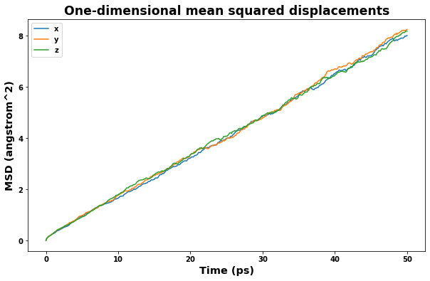
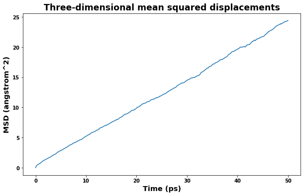
4.2.4. Plot mean squared displacement
[16]:
area_unit = f'{length_unit}^2'
time_unit = 'ps'

time = uc.get_in_units(results_dict['time_values'], time_unit)
msd_x = uc.get_in_units(results_dict['msd_x_values'], area_unit)
msd_y = uc.get_in_units(results_dict['msd_y_values'], area_unit)
msd_z = uc.get_in_units(results_dict['msd_z_values'], area_unit)
msd = uc.get_in_units(results_dict['msd_values'], area_unit)

fig = plt.figure(figsize=(10,6))
plt.title('One-dimensional mean squared displacements', size='xx-large')
plt.xlabel(f'Time ({time_unit})', size='x-large')
plt.ylabel(f'MSD ({area_unit})', size='x-large')
plt.plot(time, msd_x, label='x')
plt.plot(time, msd_y, label='y')
plt.plot(time, msd_z, label='z')
plt.legend()
plt.show()

fig = plt.figure(figsize=(10,6))
plt.title('Three-dimensional mean squared displacements', size='xx-large')
plt.xlabel(f'Time ({time_unit})', size='x-large')
plt.ylabel(f'MSD ({area_unit})', size='x-large')
plt.plot(time, msd)
plt.show()
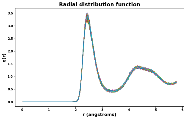
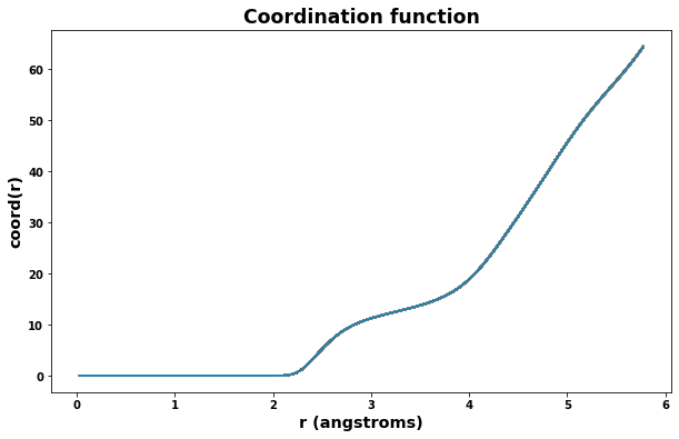
4.3. Plot radial distribution function
Radial distribution results are saved to the file rdf.txt. The class defined below will read the file and make plotting easy.
[17]:
from atomman.tools import uber_open_rmode
import pandas as pd

class RDF():
    """Class for interpreting LAMMPS rdf (radial distribution function) output files"""

    def __init__(self, rdf_file=None):

        if rdf_file is not None:
            self.read(rdf_file)

    def read(self, rdf_file):


        self.data = {}
        numvals = 0
        timeheader = 3
        with uber_open_rmode(rdf_file) as rdf_data:

            for i, line in enumerate(rdf_data):
                line = line.decode('UTF-8')

                if i == 0:
                    self.info = line[2:]
                elif i < 3:
                    continue

                elif i == timeheader:
                    terms = line.split()
                    timestep = int(terms[0])
                    numvals = int(terms[1])

                    # initialize data for the timestep
                    self.data[timestep] = pd.DataFrame({'r': np.empty(numvals),
                                                       'g': np.empty(numvals),
                                                       'coord': np.empty(numvals)})
                    timeheader += numvals + 1

                else:
                    terms = line.split()
                    j = int(terms[0]) - 1
                    self.data[timestep].loc[j, 'r'] = float(terms[1])
                    self.data[timestep].loc[j, 'g'] = float(terms[2])
                    self.data[timestep].loc[j, 'coord'] = float(terms[3])
[18]:
rdf = RDF('rdf.txt')

fig = plt.figure(figsize=(10,6))
plt.title('Radial distribution function', size='xx-large')
plt.xlabel('r (angstroms)', size='x-large')
plt.ylabel('g(r)', size='x-large')
for timeseries in rdf.data:
    plt.plot(rdf.data[timeseries].r, rdf.data[timeseries].g)
plt.show()

fig = plt.figure(figsize=(10,6))
plt.title('Coordination function', size='xx-large')
plt.xlabel('r (angstroms)', size='x-large')
plt.ylabel('coord(r)', size='x-large')
for timeseries in rdf.data:
    plt.plot(rdf.data[timeseries].r, rdf.data[timeseries].coord)
plt.show()
4.4. Look at simulation thermo results in the log.lammps file
This is a complex calculation with many components. It can be useful to check the reported thermo values of some of the earlier stages to ensure that the individual stages behaved properly.
[19]:
# The log content can be directly accessed when the calculation is done in a Python environment
log = results_dict['lammps_output']

# Or, read the info in from the log file...
#log = am.lammps.Log('log.lammps')
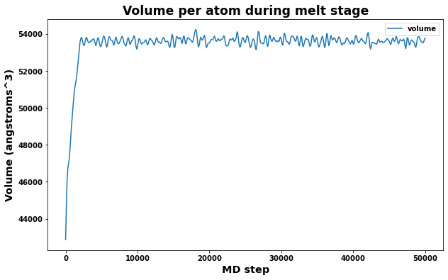
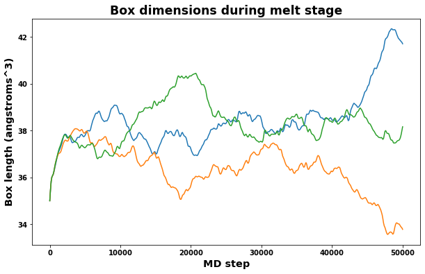
4.4.1. Check Melt stage
A quick check of volume and box dimensions during the melt stage can help reveal if the system has transformed into a liquid.
The measured volume should converge to a constant value.
The measured box dimensions should not converge to constant values.
[20]:
fig = plt.figure(figsize=(10,6))
plt.title('Volume per atom during melt stage', size='xx-large')
plt.xlabel('MD step', size='x-large')
plt.ylabel('Volume (angstroms^3)', size='x-large')
plt.plot(log.simulations[0].thermo.Step, log.simulations[0].thermo.Volume, label='volume')
plt.legend()
plt.show()

fig = plt.figure(figsize=(10,6))
plt.title('Box dimensions during melt stage', size='xx-large')
plt.xlabel('MD step', size='x-large')
plt.ylabel('Box length (angstroms^3)', size='x-large')
plt.plot(log.simulations[0].thermo.Step, log.simulations[0].thermo.Lx, label='lx')
plt.plot(log.simulations[0].thermo.Step, log.simulations[0].thermo.Ly, label='ly')
plt.plot(log.simulations[0].thermo.Step, log.simulations[0].thermo.Lz, label='lz')
plt.show()
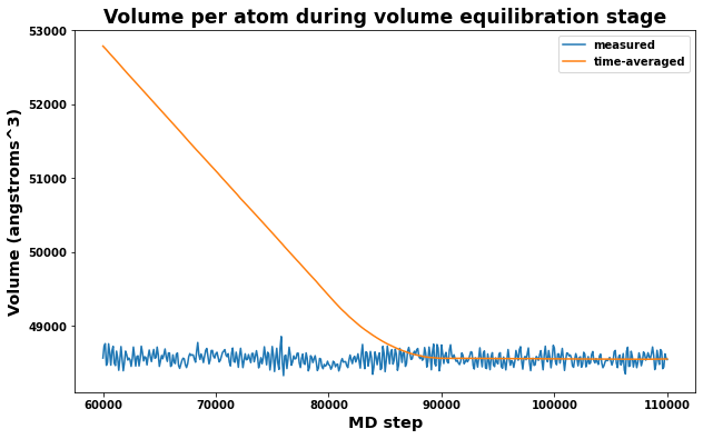
4.4.2. Volume equilibration stage
Also important is to check that the measured volume and time averaged volumes are converging appropriately for the volume equilibration stage. Note that only the last time-averaged value is used to adjust the system dimensions.
[21]:
# Plot volume and average volume during the volume equilibrate stage to check convergence
fig = plt.figure(figsize=(10,6))

plt.title('Volume per atom during volume equilibration stage', size='xx-large')
plt.xlabel('MD step', size='x-large')
plt.ylabel('Volume (angstroms^3)', size='x-large')
plt.plot(log.simulations[2].thermo.Step, log.simulations[2].thermo.Volume, label='measured')
plt.plot(log.simulations[2].thermo.Step, log.simulations[2].thermo.f_ave_vol, label='time-averaged')
plt.legend()
plt.show()